Chapter 5 Supervised Classifcation
In supervised classification, we have prior knowledge about some og the land-cover types. We need areas with identified land-cover types ti use them as training set to train the classification algotithm. In the following example we will use a Classification and Regresstion Trees (CART) classifier to predict land cover classes in the study area. We will perform the following steps: - Generate sample sites based on a reference raster - Extract alues from landsat data for the sample sites - Train the classifier using training samples - classify the landsat data using the trained model - Evaluate the accuracy of the model
5.1 Reference data
The National Land Cover Databae 2011 (NLCD 2011) is a land cover product for the USA. NLCD is a 30-m Landsat-based land cover database. It is based on a decision tree classification of circa 2011 Landsat data. It has two pairs of class vales and names that correspond to the levels of land use and land cover classification system.
First, we will load land cover data and prepare it for classification by attributing class names.
library(raster)
nlcd <- brick('data/rs/nlcd-L1.tif')
names(nlcd) <- c("nlcd2001", "nlcd2011")
# The class names and colors for plotting
nlcdclass <- c("Water", "Developed", "Barren", "Forest", "Shrubland", "Herbaceous", "Planted/Cultivated", "Wetlands")
classdf <- data.frame(classvalue1 = c(1,2,3,4,5,7,8,9), classnames1 = nlcdclass)
# Hex codes of colors
classcolor <- c("#5475A8", "#B50000", "#D2CDC0", "#38814E", "#AF963C", "#D1D182", "#FBF65D", "#C8E6F8")
# Now we ratify (RAT = "Raster Attribute Table") the ncld2011 (define RasterLayer as a categorical variable). This is helpful for plotting.
nlcd2011 <- nlcd[[2]]
nlcd2011 <- ratify(nlcd2011)
rat <- levels(nlcd2011)[[1]]
#
rat$landcover <- nlcdclass
levels(nlcd2011) <- rat
5.2 Generate sample sites
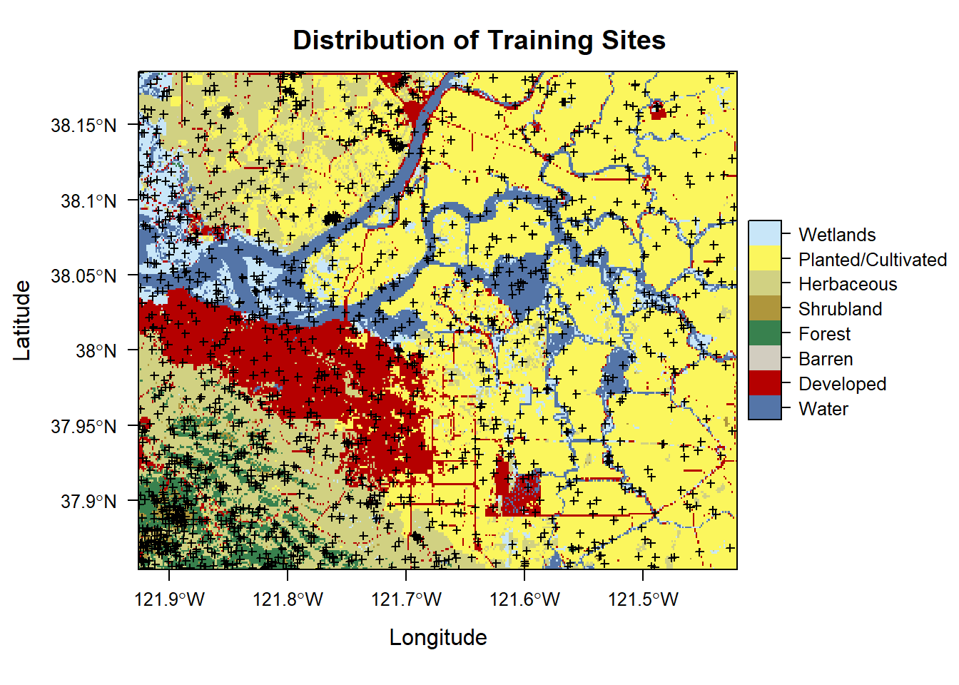
In this part We split the NLCD reference RatserLayer into training and validation sets.Before that we will spatial points of the site by ensuring equidistribution of land use classes by performing a stratified random sampling.
# set the random number generator to reproduce the results
set.seed(99)
# Sampling
samp2011 = sampleStratified(nlcd2011, size = 200, na.rm = TRUE, sp = TRUE)
samp2011
## class : SpatialPointsDataFrame
## features : 1600
## extent : -121.9257, -121.4225, 37.85415, 38.18536 (xmin, xmax, ymin, ymax)
## crs : +proj=longlat +datum=WGS84 +no_defs +ellps=WGS84 +towgs84=0,0,0
## variables : 2
## names : cell, nlcd2011
## min values : 413, 1
## max values : 2307837, 9##
## 1 2 3 4 5 7 8 9
## 200 200 200 200 200 200 200 200We can plot the sampled points to visualize the distribution of sampling locations.
## Loading required package: lattice## Loading required package: latticeExtraplt <- levelplot(nlcd2011, col.regions = classcolor, main = 'Distribution of Training Sites')
print(plt + layer(sp.points(samp2011, pch = 3, cex = 0.5, col = 1)))
5.3 Extract values for sites
We load the Landsat data
landsat5 <- stack('data/rs/centralvalley-2011LT5.tif')
names(landsat5) <- c('blue', 'green', 'red', 'NIR', 'SWIR1', 'SWIR2')
We extract the raster values (for different band length of landsat data) corresponding to the sampled points with identified land cover classes. Then we create a dataframe containing the band values (which are our predictor variables) and the corresponding classes (which is our reponse variable)
sampvals <- extract(landsat5, samp2011, df = TRUE)
# sampvals no longer has the spatial information. To keep the spatial information you use `sp=TRUE` argument in the `extract` function.
# drop the ID column
sampvals <- sampvals[, -1]
# combine the class information with extracted values
sampdata <- data.frame(classvalue = samp2011@data$nlcd2011, sampvals)
5.4 Train the classifier
library(rpart)
# Train the model
cart <- rpart(as.factor(classvalue)~., data=sampdata, method = 'class', minsplit = 5)
# print(model.class)
# Plot the trained classification tree
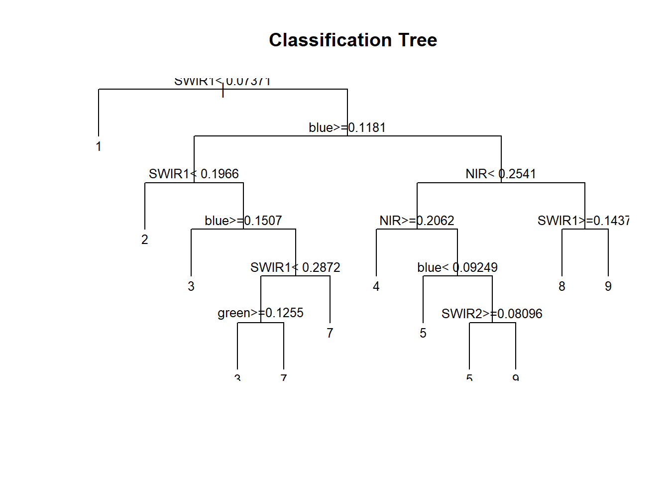
plot(cart, uniform=TRUE, main="Classification Tree")
text(cart, cex = 0.8)
The classification tree plot shows the classvalues at the leaf nodes.
5.5 Classify
Now we have a trained classification model that we can use to classify the cells in the landsat rasterstack.
# Now predict the subset data based on the model; prediction for entire area takes longer time
pr2011 <- predict(landsat5, cart, type='class')
pr2011
## class : RasterLayer
## dimensions : 1230, 1877, 2308710 (nrow, ncol, ncell)
## resolution : 0.0002694946, 0.0002694946 (x, y)
## extent : -121.9258, -121.42, 37.85402, 38.1855 (xmin, xmax, ymin, ymax)
## crs : +proj=longlat +datum=WGS84 +no_defs +ellps=WGS84 +towgs84=0,0,0
## source : memory
## names : layer
## values : 1, 9 (min, max)
## attributes :
## ID value
## from: 1 1
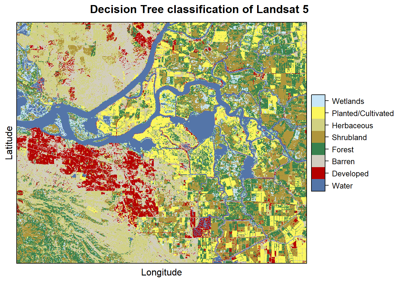
## to : 8 9We can plot the classification results
pr2011 <- ratify(pr2011)
rat <- levels(pr2011)[[1]]
rat$legend <- classdf$classnames
levels(pr2011) <- rat
levelplot(pr2011, maxpixels = 1e6,
          col.regions = classcolor,
          scales=list(draw=FALSE),
          main = "Decision Tree classification of Landsat 5")
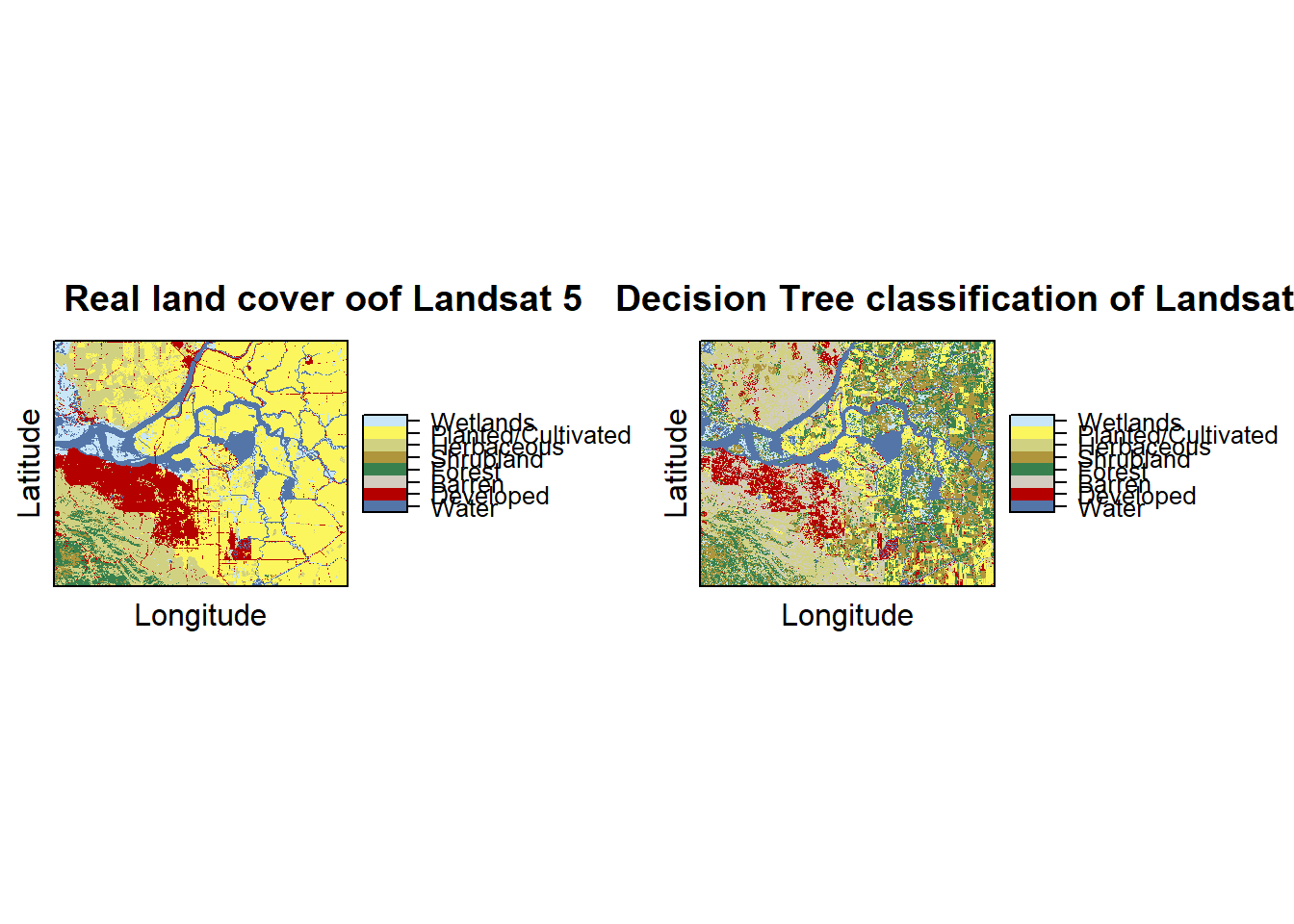
We can plot side by side the real and predicted land cover in order to assess the classification model accuracy
plot1 = levelplot(nlcd2011, maxpixels = 1e6,
          col.regions = classcolor,
          scales=list(draw=FALSE),
          main = "Real land cover oof Landsat 5")
plot2 = levelplot(pr2011, maxpixels = 1e6,
          col.regions = classcolor,
          scales=list(draw=FALSE),
          main = "Decision Tree classification of Landsat 5")

library(gridExtra)
grid.arrange(plot1,plot2, ncol=2)
5.6 Model Evaluation
Now we have to assess the accuracy of the model. Two metrics are widely used in remote sensing: “overall accuracy” and “kappa”.
5.6.1 K-fold cross validation
We will use k-fold cross validation for the model evaluation. This technique consists on splitting the data to fit the model into k groups. In turn, one of the groups will be used for model testing, while the rest of the data is used for model training.
## j
##   1   2   3   4   5
## 320 320 320 320 320
Now we trainand test the model five times, each time computing a confusion matrix that we store in a list.
x <- list()
for (k in 1:5) {
  train <- sampdata[j!= k, ]
  test <- sampdata[j == k, ]
  cart <- rpart(as.factor(classvalue)~., data=train, method = 'class', minsplit = 5)
  pclass <- predict(cart, test, type='class')
  # create a data.frame using the reference and prediction
  x[[k]] <- cbind(test$classvalue, as.integer(pclass))
}
Now we combine the five list elements in a single dataframe
y <- do.call(rbind, x)
y <- data.frame(y)
colnames(y) <- c('observed', 'predicted')
conmat <- table(y)
# change the name of the classes
colnames(conmat) <- classdf$classnames
rownames(conmat) <- classdf$classnames
conmat
## predicted
## observed Water Developed Barren Forest Shrubland Herbaceous
## Water 175 6 0 3 0 0
## Developed 2 90 51 8 10 22
## Barren 7 39 82 4 19 38
## Forest 0 2 1 106 57 1
## Shrubland 0 3 5 59 102 12
## Herbaceous 0 9 36 10 27 109
## Planted/Cultivated 0 7 11 34 42 19
## Wetlands 18 10 6 36 29 5
## predicted
## observed Planted/Cultivated Wetlands
## Water 7 9
## Developed 11 6
## Barren 5 6
## Forest 6 27
## Shrubland 12 7
## Herbaceous 8 1
## Planted/Cultivated 69 18
## Wetlands 33 635.6.2 Overall accuracy
## [1] 1600# number of correctly classified cases per class
diag <- diag(conmat)
# Overall Accuracy
OA <- sum(diag) / n
OA## [1] 0.49755.6.3 Kappa statistic
# observed (true) cases per class
rowsums <- apply(conmat, 1, sum)
p <- rowsums / n
# predicted cases per class
colsums <- apply(conmat, 2, sum)
q <- colsums / n
expAccuracy <- sum(p*q)
kappa <- (OA - expAccuracy) / (1 - expAccuracy)
kappa
## [1] 0.42571435.6.4 Producer and user accuracy
# Producer accuracy
PA <- diag / colsums
# User accuracy
UA <- diag / rowsums
outAcc <- data.frame(producerAccuracy = PA, userAccuracy = UA)
outAcc
## producerAccuracy userAccuracy
## Water 0.8663366 0.875
## Developed 0.5421687 0.450
## Barren 0.4270833 0.410
## Forest 0.4076923 0.530
## Shrubland 0.3566434 0.510
## Herbaceous 0.5291262 0.545
## Planted/Cultivated 0.4569536 0.345
## Wetlands 0.4598540 0.315