Chapter 3 ARMA Time Series modeling
3.1 Auto-Regressive Time Series model
The Auto-Regressive (AR) model can be interpreted as a simple linear regression where each observation \(x(t)\) is regressed on the previous observation \(x(t-1)\).
It can be formulated with the following equation known as AR(1) formulation:
\[x(t) = \alpha \times x(t-1) + error(t)\]
The equation denotes that the current instance is dependant on the previous one with an alpha coefficient which we seek to minimize the error function. If \(\alpha = 0\) then \(x(t)\) is simply white noise. Large \(\alpha\) show a high correlation and negative values of \(\alpha\) result in oscillatory time series.
- Fitting an AR model: We can use the command
arima()in order to fit an AR model to a time series. An AR model is an ARIMA model with order (1,0,0).
#Fitting the AR Model to the time series
AR <- arima(AirPassengers, order = c(1,0,0))
print(AR)
##
## Call:
## arima(x = AirPassengers, order = c(1, 0, 0))
##
## Coefficients:
## ar1 intercept
## 0.9646 278.4649
## s.e. 0.0214 67.1141
##
## sigma^2 estimated as 1119: log likelihood = -711.09, aic = 1428.18#plotting the series along with the fitted values
ts.plot(AirPassengers)
AR_fit <- AirPassengers - residuals(AR)
points(AR_fit, type = "l", col = 2, lty = 2)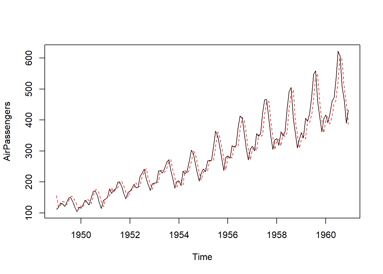
- Forecasting using an AR model: We can make forecasts using the estimated AR model using the command
predictwhich gives us the predicted value ($pred) and standard error of the forecast ($se).
#Using predict() to make a 1-step forecast
predict_AR <- predict(AR)
predict_AR
## $pred
## Jan
## 1961 426.5698
##
## $se
## Jan
## 1961 33.44577#Obtaining the 1-step forecast using $pred[1]
predict_AR$pred[1]## [1] 426.5698# predicting 10 step forecats
predict(AR, n.ahead = 10)## $pred
## Jan Feb Mar Apr May Jun Jul Aug
## 1961 426.5698 421.3316 416.2787 411.4045 406.7027 402.1672 397.7921 393.5717
## Sep Oct
## 1961 389.5006 385.5735
##
## $se
## Jan Feb Mar Apr May Jun Jul Aug
## 1961 33.44577 46.47055 55.92922 63.47710 69.77093 75.15550 79.84042 83.96535
## Sep Oct
## 1961 87.62943 90.90636We can visualize the forecasts with 95% prediction intervals
ts.plot(AirPassengers, xlim = c(1949, 1961))
AR_forecast <- predict(AR, n.ahead = 10)$pred
AR_forecast_se <- predict(AR, n.ahead = 10)$se
points(AR_forecast, type = "l", col = 2)
points(AR_forecast - 2*AR_forecast_se, type = "l", col = 2, lty = 2)
points(AR_forecast + 2*AR_forecast_se, type = "l", col = 2, lty = 2)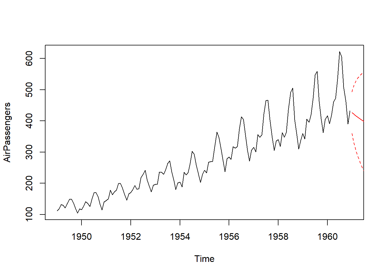
3.2 Moving Average Time Series Model
The Moving Average (MA) model has a regression llike form, but each observation is regressed on the previous innovation, which is not actually observed. A weighted sum of previous and current noise is called Moving Average (MA) model. It can be interpreted as: each observation \(x(t)\) is regressed on previous noise \(error(t-1)\). It can be formulated with the following equation known as MA(1) formulation:
\[x(t) = \beta \times error(t-1) + error(t)\] The \(\beta\) is a coefficient which we seek to mimize the error function.
- Fitting an AR model: We can use the command
arima()in order to fit a MA model to a time series. A MA model is an ARIMA model with order (0,0,1).
#Fitting the MA model to AirPassengers
MA <- arima(AirPassengers, order = c(0,0,1))
print(MA)
##
## Call:
## arima(x = AirPassengers, order = c(0, 0, 1))
##
## Coefficients:
## ma1 intercept
## 0.9642 280.6464
## s.e. 0.0214 10.5788
##
## sigma^2 estimated as 4205: log likelihood = -806.43, aic = 1618.86#plotting the series along with the MA fitted values
ts.plot(AirPassengers)
MA_fit <- AirPassengers - resid(MA)
points(MA_fit, type = "l", col = 2, lty = 2)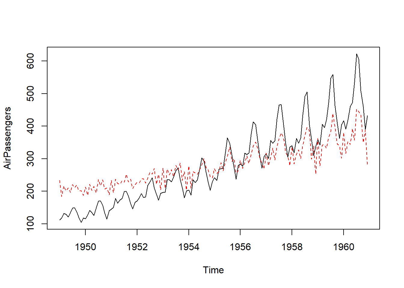
- Forecasting using an AR model: We can make forecasts using the estimated AR model using the command
predictwhich gives us the predicted value ($pred) and standard error of the forecast ($se).
# Making a 1-step through 10-step forecast based on MA
predict(MA,n.ahead=10)
## $pred
## Jan Feb Mar Apr May Jun Jul Aug
## 1961 425.1049 280.6464 280.6464 280.6464 280.6464 280.6464 280.6464 280.6464
## Sep Oct
## 1961 280.6464 280.6464
##
## $se
## Jan Feb Mar Apr May Jun Jul Aug
## 1961 64.84895 90.08403 90.08403 90.08403 90.08403 90.08403 90.08403 90.08403
## Sep Oct
## 1961 90.08403 90.08403We can visualize the forecasts with 95% prediction intervals
#Plotting the AIrPAssenger series plus the forecast and 95% prediction intervals
ts.plot(AirPassengers, xlim = c(1949, 1961))
MA_forecasts <- predict(MA, n.ahead = 10)$pred
MA_forecast_se <- predict(MA, n.ahead = 10)$se
points(MA_forecasts, type = "l", col = 2)
points(MA_forecasts - 2*MA_forecast_se, type = "l", col = 2, lty = 2)
points(MA_forecasts + 2*MA_forecast_se, type = "l", col = 2, lty = 2)
3.3 Model selection: AR or MA
We can you godness of fit in order to choose the more appropriate model. Two metrics are commonly used in time series model: Akaike Information Criterion (AIC) and Bayesian Information Criterion (BIC). A lower value indicates a better fitting model. These two indicators penalize models with more estimated parameters in order to avoid overfitting.
- Akaike Information Criterion (AIC):
- Bayesian Information Criterion (BIC):
# Compute AIC of AR model
AIC(AR)
## [1] 1428.179# Compute AIC of MA model
AIC(MA)## [1] 1618.863# Compute BIC of AR model
BIC(AR)## [1] 1437.089# Compute BIC of MA model
BIC(MA)## [1] 1627.772Based on the results, we can select the AR model since it gives lower value of AIC and BIC.