Chapter 4 Deep learning for computer vision

4.1 Image classification with Keras

We will see here a simple image classification example using Keras based on the MNIST dataset.

4.1.1 download and prepare the data

library(keras)

# load data
mnist = dataset_mnist()
# rescale the data
mnist$train$x = mnist$train$x / 255
mnist$test$x = mnist$test$x / 255
# dimensions
dim(mnist$train[[1]])

## [1] 60000    28    28

dim(mnist$test[[1]])

## [1] 10000    28    28

4.1.2 Build the model

model = keras_model_sequential() %>% 
  layer_flatten(input_shape = c(28,28)) %>%  # we have to specify the input dimensions for the first layer. In our case we have imahes of 28x28
  layer_dense(units = 128, activation = "relu") %>% 
  layer_dropout(0.2) %>% 
  layer_dense(10, activation = "softmax")

summary(model)

## Model: "sequential_1"
## ________________________________________________________________________________
## Layer (type)                        Output Shape                    Param #     
## ================================================================================
## flatten (Flatten)                   (None, 784)                     0           
## ________________________________________________________________________________
## dense_6 (Dense)                     (None, 128)                     100480      
## ________________________________________________________________________________
## dropout (Dropout)                   (None, 128)                     0           
## ________________________________________________________________________________
## dense_7 (Dense)                     (None, 10)                      1290        
## ================================================================================
## Total params: 101,770
## Trainable params: 101,770
## Non-trainable params: 0
## ________________________________________________________________________________

4.1.3 Compile the model

model %>% 
  compile(
    loss = "sparse_categorical_crossentropy",
    optimizer = "adam",
    metrics = "accuracy"
  )

4.1.4 Fit the model

model %>% 
  fit(
    x = mnist$train$x, y = mnist$train$y,
    epochs = 5, # iterations
    validation_split = 0.3, # fraction of the training data to be used as validation data
    verbose = 2 # 0= silent, 1=progress bar,2=one line per epoch
  )

4.1.5 Make predictions

predictions <- predict(model, mnist$test$x)
head(predictions, 2)

##              [,1]         [,2]         [,3]         [,4]         [,5]
## [1,] 3.529128e-06 5.023255e-08 6.188818e-06 0.0011937367 4.015424e-10
## [2,] 3.211236e-08 3.743406e-03 9.961239e-01 0.0001220347 1.333065e-11
##              [,6]         [,7]         [,8]        [,9]        [,10]
## [1,] 2.261655e-08 1.261817e-12 9.987532e-01 6.27417e-07 4.259534e-05
## [2,] 3.711051e-06 2.744141e-07 2.890228e-13 6.79126e-06 9.612983e-15

predictions <- predict_classes(model, mnist$test$x)
head(predictions, 2)

## [1] 7 2

predictions <- predict_proba(model, mnist$test$x)
head(predictions, 2)

##              [,1]         [,2]         [,3]         [,4]         [,5]
## [1,] 3.529128e-06 5.023255e-08 6.188818e-06 0.0011937367 4.015424e-10
## [2,] 3.211236e-08 3.743406e-03 9.961239e-01 0.0001220347 1.333065e-11
##              [,6]         [,7]         [,8]        [,9]        [,10]
## [1,] 2.261655e-08 1.261817e-12 9.987532e-01 6.27417e-07 4.259534e-05
## [2,] 3.711051e-06 2.744141e-07 2.890228e-13 6.79126e-06 9.612983e-15

4.1.6 Evaluate the model

model %>% 
  evaluate(mnist$test$x, mnist$test$y, verbose = 0)

## $loss
## [1] 0.09325283
## 
## $accuracy
## [1] 0.9727

4.1.7 Save the model

save_model_tf(object = model, filepath = "D:/image/DeepLearning-ComputerVision/models/mnist")
save_model_hdf5(object = model, filepath = "D:/image/DeepLearning-ComputerVision/models/Mnist_hdf5")

4.1.8 reload the model

reloaded_model <- load_model_tf("D:/image/DeepLearning-ComputerVision/models/mnist")
reloaded_model_hdf5 = load_model_hdf5("D:/image/DeepLearning-ComputerVision/models/Mnist_hdf5")

predictions_reloaded = predict(reloaded_model_hdf5, mnist$test$x)
head(predictions_reloaded)

##              [,1]         [,2]         [,3]         [,4]         [,5]
## [1,] 3.529128e-06 5.023255e-08 6.188818e-06 1.193737e-03 4.015424e-10
## [2,] 3.211236e-08 3.743406e-03 9.961239e-01 1.220347e-04 1.333065e-11
## [3,] 2.589487e-07 9.985394e-01 1.053339e-04 2.851183e-05 2.373429e-05
## [4,] 9.996665e-01 2.241493e-08 1.531596e-05 1.124228e-06 9.338348e-07
## [5,] 1.878520e-06 4.146345e-08 9.855919e-06 3.727743e-06 9.916103e-01
## [6,] 4.119136e-10 9.997892e-01 7.075888e-07 5.189237e-07 1.103822e-06
##              [,6]         [,7]         [,8]         [,9]        [,10]
## [1,] 2.261655e-08 1.261817e-12 9.987532e-01 6.274170e-07 4.259534e-05
## [2,] 3.711051e-06 2.744141e-07 2.890228e-13 6.791260e-06 9.612983e-15
## [3,] 2.637429e-05 2.095207e-05 1.111350e-03 1.431736e-04 8.765668e-07
## [4,] 2.384290e-06 2.039706e-04 8.382809e-05 2.111165e-08 2.596046e-05
## [5,] 1.645499e-06 2.099444e-05 3.041392e-05 1.886919e-06 8.319193e-03
## [6,] 1.491091e-08 1.555326e-08 2.077410e-04 8.532269e-07 1.392535e-08

head(predictions)

##              [,1]         [,2]         [,3]         [,4]         [,5]
## [1,] 3.529128e-06 5.023255e-08 6.188818e-06 1.193737e-03 4.015424e-10
## [2,] 3.211236e-08 3.743406e-03 9.961239e-01 1.220347e-04 1.333065e-11
## [3,] 2.589487e-07 9.985394e-01 1.053339e-04 2.851183e-05 2.373429e-05
## [4,] 9.996665e-01 2.241493e-08 1.531596e-05 1.124228e-06 9.338348e-07
## [5,] 1.878520e-06 4.146345e-08 9.855919e-06 3.727743e-06 9.916103e-01
## [6,] 4.119136e-10 9.997892e-01 7.075888e-07 5.189237e-07 1.103822e-06
##              [,6]         [,7]         [,8]         [,9]        [,10]
## [1,] 2.261655e-08 1.261817e-12 9.987532e-01 6.274170e-07 4.259534e-05
## [2,] 3.711051e-06 2.744141e-07 2.890228e-13 6.791260e-06 9.612983e-15
## [3,] 2.637429e-05 2.095207e-05 1.111350e-03 1.431736e-04 8.765668e-07
## [4,] 2.384290e-06 2.039706e-04 8.382809e-05 2.111165e-08 2.596046e-05
## [5,] 1.645499e-06 2.099444e-05 3.041392e-05 1.886919e-06 8.319193e-03
## [6,] 1.491091e-08 1.555326e-08 2.077410e-04 8.532269e-07 1.392535e-08

4.2 Introduction to Convolution Neural Networks

4.2.1 Example

The following lines of code show a basic convnet model structure. It is a stack of layer_conv_2d and layer_max_pooling_2d layers.

library(keras)

model = keras_model_sequential() %>% 
  layer_conv_2d(filters = 32, kernel_size = c(3,3), activation = "relu", input_shape = c(28,28,1)) %>% 
  layer_max_pooling_2d(pool_size = c(2,2)) %>% 
  layer_conv_2d(filters = 64, kernel_size = c(3,3), activation = "relu") %>% 
  layer_max_pooling_2d(pool_size = c(2,2)) %>% 
  layer_conv_2d(filters = 64, kernel_size = c(3,3), activation = "relu")

A convnet takes as input tensors of shape (image_height, image_width, image_channels). In the example above, we configured the convnet to process inputs of size (28, 28, 1) by specifying the argument input_shape = c(28,28,1).

Let’s show the model architecture

model

## Model
## Model: "sequential_2"
## ________________________________________________________________________________
## Layer (type)                        Output Shape                    Param #     
## ================================================================================
## conv2d (Conv2D)                     (None, 26, 26, 32)              320         
## ________________________________________________________________________________
## max_pooling2d (MaxPooling2D)        (None, 13, 13, 32)              0           
## ________________________________________________________________________________
## conv2d_1 (Conv2D)                   (None, 11, 11, 64)              18496       
## ________________________________________________________________________________
## max_pooling2d_1 (MaxPooling2D)      (None, 5, 5, 64)                0           
## ________________________________________________________________________________
## conv2d_2 (Conv2D)                   (None, 3, 3, 64)                36928       
## ================================================================================
## Total params: 55,744
## Trainable params: 55,744
## Non-trainable params: 0
## ________________________________________________________________________________

Then we feed the last output tensor (of shape (3,3,64)) into a densly connected classifier network. Since the classifiers process vectors (1D), we need to flatten the 3D outputs to 1D before adding dense layers on top.

model = model %>% 
  layer_flatten() %>% 
  layer_dense(units = 64, activation = "relu") %>% 
  layer_dense(units = 10, activation = "softmax")
model

## Model
## Model: "sequential_2"
## ________________________________________________________________________________
## Layer (type)                        Output Shape                    Param #     
## ================================================================================
## conv2d (Conv2D)                     (None, 26, 26, 32)              320         
## ________________________________________________________________________________
## max_pooling2d (MaxPooling2D)        (None, 13, 13, 32)              0           
## ________________________________________________________________________________
## conv2d_1 (Conv2D)                   (None, 11, 11, 64)              18496       
## ________________________________________________________________________________
## max_pooling2d_1 (MaxPooling2D)      (None, 5, 5, 64)                0           
## ________________________________________________________________________________
## conv2d_2 (Conv2D)                   (None, 3, 3, 64)                36928       
## ________________________________________________________________________________
## flatten_1 (Flatten)                 (None, 576)                     0           
## ________________________________________________________________________________
## dense_8 (Dense)                     (None, 64)                      36928       
## ________________________________________________________________________________
## dense_9 (Dense)                     (None, 10)                      650         
## ================================================================================
## Total params: 93,322
## Trainable params: 93,322
## Non-trainable params: 0
## ________________________________________________________________________________

We see that the (3,3,64) ouputs are flattened into vectors of shape (576) before being feeded to dense layers.

Now let’s train the convnet on the MNIST digits data.

mnist = dataset_mnist()
c(c(train_images, train_labels), c(test_images, test_labels)) %<-% mnist
train_images = array_reshape(train_images, c(60000, 28, 28, 1))
train_images = train_images / 255
test_images = array_reshape(test_images, c(10000, 28, 28, 1))
test_images = test_images / 255
train_labels = to_categorical(train_labels)
test_labels = to_categorical(test_labels)
model %>%  compile(
  optimizer = "rmsprop",
  loss = "categorical_crossentropy",
  metrics = c("accuracy")
)

model %>% fit(
  train_images, train_labels,
  epochs = 5, batch_size = 64
)

let’s evaluate the model on the test data

results = model %>% evaluate(test_images, test_labels)
results

## $loss
## [1] 0.03118547
## 
## $accuracy
## [1] 0.9914

4.2.2 The convolution operation

The objective of convolution layers is to learn local patterns. They have two main charecteristics:

They are translation invariant
They can learn spatial hierarchies of pattterns

In te MNIST example, the first convolution layer takes a feature map of size (28,28,1) and outputs a feature map of size (26,26,32): it computes 32 filters over its inputs. Each output contains a 26x26 grid of values representing a response map of the filter over different locations of the input. Convolutions are defined based on two main parameters:

Size of patches extracted from the inputs: We often use 3 x 3 or 5 x 5 patches.
Depth of the output feature map: It represents the number of filters computes by the convolution. In the example, we started with a depth of 32 and ended with a depth of 64.

The convolutio works by sliding windows of size 3x3 or 5x5 over the input feature map and extracting at every location the patch of features. Each patch is then transformed in a 1D vector by computing a tensor product with the weight matrix called convolution kernel. We remark that the output width and height can be different from the input widthand height because of border effects and used strides.

4.2.2.1 Border effects and padding

Border effects make that the output size feature map of convolution is less large that the input feature map (in the previous example from 28x28 to 26x26). We can avoid this effect by using padding, which consists on adding an appropriate number of rows and columns on each side of the input feature map to make it possible to fit center convolution windows around every input tile.

4.2.2.2 Convolution strides

The stride represents the distance between two successive windows.

4.2.3 The max-pooling operation

Max pooling consists of extracting windows from the input feature maps and outputting the max value of each channel. It is usually done with 2x2 windows and stride of 2, in order to downsample the feature maps by a factor of 2. This operation helps in reducing he number of feature-map coeficients to process.

4.3 Architectures of CNN

LeNet-5 (1998) It has 2 convolutional with average pooling and 3 fully-connected layers. The activation function is Tanh.

LeNet-5 (https://towardsdatascience.com/illustrated-10-cnn-architectures-95d78ace614d)

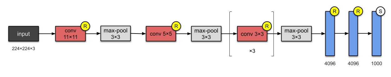
AlexNet (2012)

AlexNet has 8 layers: 5 convolutional with maxpooling and 3 fully connected. The activation function is ReLU.

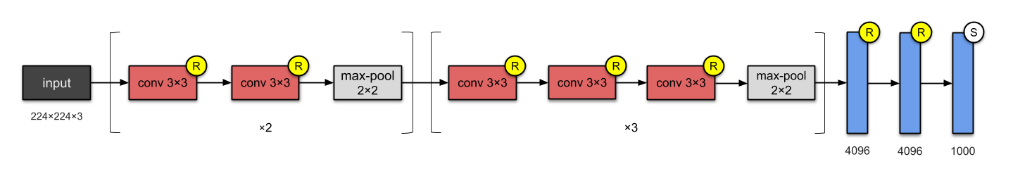
AlexNet (https://towardsdatascience.com/illustrated-10-cnn-architectures-95d78ace614d)

VGG-16 (2014)

It has 13 convolutional and 3 fully connected layers.

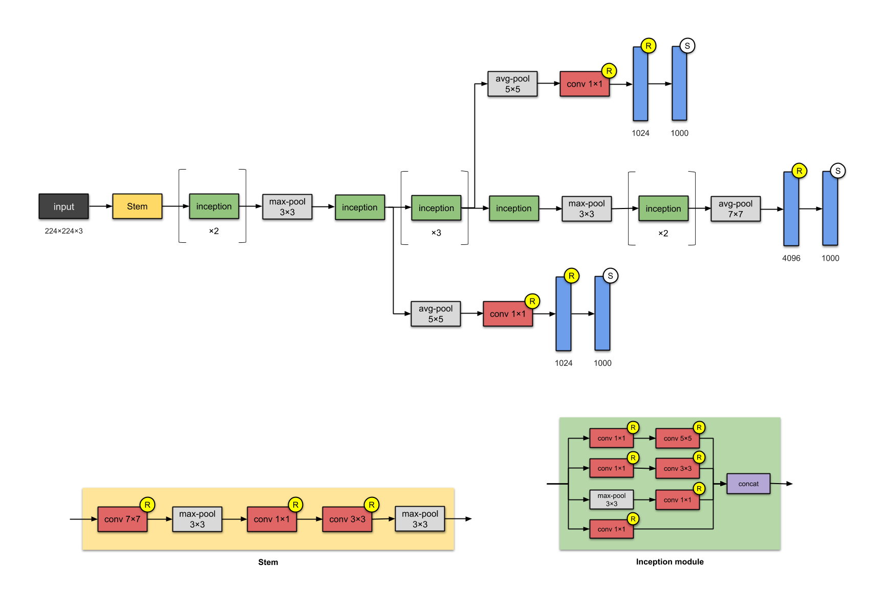
VGG-16 (https://towardsdatascience.com/illustrated-10-cnn-architectures-95d78ace614d)

Inception v1 - GoogleNet (2014)

It is a Network in Network approach.

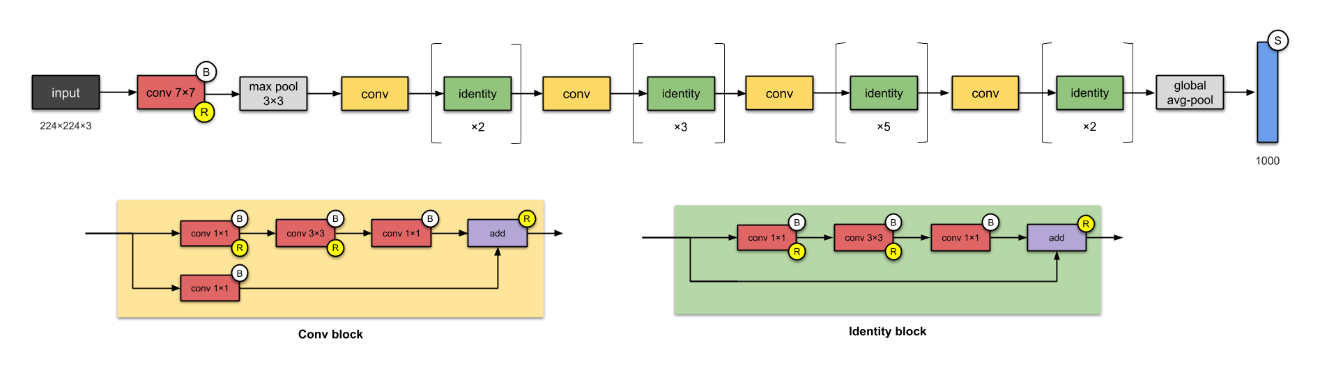
Inception v1 (https://towardsdatascience.com/illustrated-10-cnn-architectures-95d78ace614d)

ResNet-50 (2015)

ResNet-50 (https://towardsdatascience.com/illustrated-10-cnn-architectures-95d78ace614d)

Xception (2016)

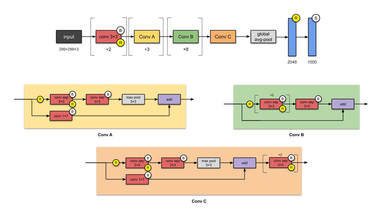
Xception (https://towardsdatascience.com/illustrated-10-cnn-architectures-95d78ace614d)

DenseNet
MobileNet

4.4 Classifcation examples

4.4.1 Dataset: Dog VS Cats

4.4.1.1 Downloading data

We will use the cats vs dogs dataset from kaggle. It contains 25,000 images of dogs and cates (12,500 for each class). After downloading the data we will create a new dataset containing three subsets: a training set with 1,000 samples of each class, a validation set with 500 samples of each class, and a test set with 500 samples of each class.

original_dataset_dir = "D:/image/DeepLearning-ComputerVision/data/dogs-vs-cats/train/train"

# ----------------------- Create base directories
# base_dir
base_dir = "D:/image/DeepLearning-ComputerVision/data/cats_and_dogs_small"
dir.create(base_dir)
# train_dir
train_dir = file.path(base_dir, "train")
dir.create(train_dir)
# validation_dir
validation_dir = file.path(base_dir, "validation")
dir.create(validation_dir)
# test_dir
test_dir = file.path(base_dir, "test")
dir.create(test_dir)

# ----------------------- train directories
# train_cats_dir
train_cats_dir = file.path(train_dir, "cats")
dir.create(train_cats_dir)
# train_dogs_dir
train_dogs_dir = file.path(train_dir, "dogs")
dir.create(train_dogs_dir)

# ----------------------- validation directories
# validation_cats_dir
validation_cats_dir = file.path(validation_dir, "cats")
dir.create(validation_cats_dir)
# validation_dogs_dir
validation_dogs_dir = file.path(validation_dir, "dogs")
dir.create(validation_dogs_dir)

# ----------------------- test directories
# test_cats_dir
test_cats_dir = file.path(test_dir, "cats")
dir.create(test_cats_dir)
# test_dogs_dir
test_dogs_dir = file.path(test_dir, "dogs")
dir.create(test_dogs_dir)

# ----------------------- copy and rename files
# ---------- cats
# train_cats_dir
fnames = paste0("cat.",1:1000, ".jpg")
file.copy(file.path(original_dataset_dir, fnames),
          file.path(train_cats_dir))
# validation_cats_dir
fnames = paste0("cat.",1001:1500, ".jpg")
file.copy(file.path(original_dataset_dir, fnames),
          file.path(validation_cats_dir))
# test_cats_dir
fnames = paste0("cat.",1501:2000, ".jpg")
file.copy(file.path(original_dataset_dir, fnames),
          file.path(test_cats_dir))
# ---------- dogs
# train_dogs_dir
fnames = paste0("dog.",1:1000, ".jpg")
file.copy(file.path(original_dataset_dir, fnames),
          file.path(train_dogs_dir))
# validation_dogs_dir
fnames = paste0("dog.",1001:1500, ".jpg")
file.copy(file.path(original_dataset_dir, fnames),
          file.path(validation_dogs_dir))
# test_dogs_dir
fnames = paste0("dog.",1501:2000, ".jpg")
file.copy(file.path(original_dataset_dir, fnames),
          file.path(test_dogs_dir))

# check
cat("total training cat images:", length(list.files(train_cats_dir)), "\n")
cat("total training dog images:", length(list.files(train_dogs_dir)), "\n")

cat("total validation cat images:", length(list.files(validation_cats_dir)), "\n")
cat("total validation dog images:", length(list.files(validation_dogs_dir)), "\n")

cat("total test cat images:", length(list.files(test_cats_dir)), "\n")
cat("total test dog images:", length(list.files(test_dogs_dir)), "\n")

4.4.1.2 Building the network

library(keras)
model = keras_model_sequential() %>% 
  layer_conv_2d(filters = 32, kernel_size = c(3,3), activation = "relu", input_shape = c(150,150,3)) %>% 
  layer_max_pooling_2d(pool_size = c(2,2)) %>% 
  layer_conv_2d(filters = 64, kernel_size = c(3,3), activation = "relu") %>% 
  layer_max_pooling_2d(pool_size = c(2,2)) %>% 
  layer_conv_2d(filters = 128, kernel_size = c(3,3), activation = "relu") %>% 
  layer_max_pooling_2d(pool_size = c(2,2)) %>%
  layer_conv_2d(filters = 128, kernel_size = c(3,3), activation = "relu") %>% 
  layer_max_pooling_2d(pool_size = c(2,2)) %>%
  layer_flatten() %>% 
  layer_dense(units = 512, activation = "relu") %>% 
  layer_dense(units = 1, activation = "sigmoid") 

summary(model)

## Model: "sequential_3"
## ________________________________________________________________________________
## Layer (type)                        Output Shape                    Param #     
## ================================================================================
## conv2d_3 (Conv2D)                   (None, 148, 148, 32)            896         
## ________________________________________________________________________________
## max_pooling2d_2 (MaxPooling2D)      (None, 74, 74, 32)              0           
## ________________________________________________________________________________
## conv2d_4 (Conv2D)                   (None, 72, 72, 64)              18496       
## ________________________________________________________________________________
## max_pooling2d_3 (MaxPooling2D)      (None, 36, 36, 64)              0           
## ________________________________________________________________________________
## conv2d_5 (Conv2D)                   (None, 34, 34, 128)             73856       
## ________________________________________________________________________________
## max_pooling2d_4 (MaxPooling2D)      (None, 17, 17, 128)             0           
## ________________________________________________________________________________
## conv2d_6 (Conv2D)                   (None, 15, 15, 128)             147584      
## ________________________________________________________________________________
## max_pooling2d_5 (MaxPooling2D)      (None, 7, 7, 128)               0           
## ________________________________________________________________________________
## flatten_2 (Flatten)                 (None, 6272)                    0           
## ________________________________________________________________________________
## dense_10 (Dense)                    (None, 512)                     3211776     
## ________________________________________________________________________________
## dense_11 (Dense)                    (None, 1)                       513         
## ================================================================================
## Total params: 3,453,121
## Trainable params: 3,453,121
## Non-trainable params: 0
## ________________________________________________________________________________

For the compilation, we will use the RMSprop optimizer. Because the network ended with a sngle sigmoid unit, we will use binary crossentropy as the loss.

model %>%  compile(
  loss = "binary_crossentropy",
  optimizer = optimizer_rmsprop(lr = 0.001),
  metrics = c("acc")
)

4.4.1.3 Data preprocessing

We need to preprocess the image data before feeding the network: decode the JPEG content to RGB grids of pixels, convert them into floating-point tensors, and rescaling the pixel values from [0,255] to [0,1] interval. Keras provides some image processing tools like image_data_generator function that turn auomatically image files on disk into batches of preprocessed tnesors.

# specify dir
train_dir = "D:/image/DeepLearning-ComputerVision/data/cats_and_dogs_small/train"
validation_dir = "D:/image/DeepLearning-ComputerVision/data/cats_and_dogs_small/validation"

# rescale all images bu 1/255
train_datagen = image_data_generator(rescale = 1/255)
validation_datagen = image_data_generator(rescale = 1/255)

train_generator = flow_images_from_directory(
  train_dir, # Traget directory
  train_datagen, # training data generator
  target_size = c(150, 150), # resize all images to 150 x 150
  batch_size = 20,
  class_mode = "binary" # because we use binary_crossentropy loss
)

validation_generator = flow_images_from_directory(
  validation_dir,
  validation_datagen,
  target_size = c(150, 150),
  batch_size = 20,
  class_mode = "binary"
)

The output of these generators constists on batches of 150x150 RGB iages and binary labels. Each batch contains 20 samples (batch size).

batch = generator_next(train_generator)
str(batch)

## List of 2
##  $ : num [1:20, 1:150, 1:150, 1:3] 0.749 0.592 0.392 1 0.251 ...
##  $ : num [1:20(1d)] 0 0 1 1 0 1 1 0 1 1 ...

We use the fit_generator function to fit the model using the generator. The fitting process needs to know how many samples to draw from the genrator before declaring an epoch over. In this example, we have batches of 20 amples, so we need 100 batches to process the whole 2000 samples. We need to specify the same thing for the validation data. Since we have 1000 validation samples, we need 50 validation steps of batches of 20 images.

history = model %>% fit_generator(
  train_generator,
  steps_per_epoch = 100,
  epochs = 5,
  validation_data = validation_generator,
  validation_steps = 50
)

We can save our model

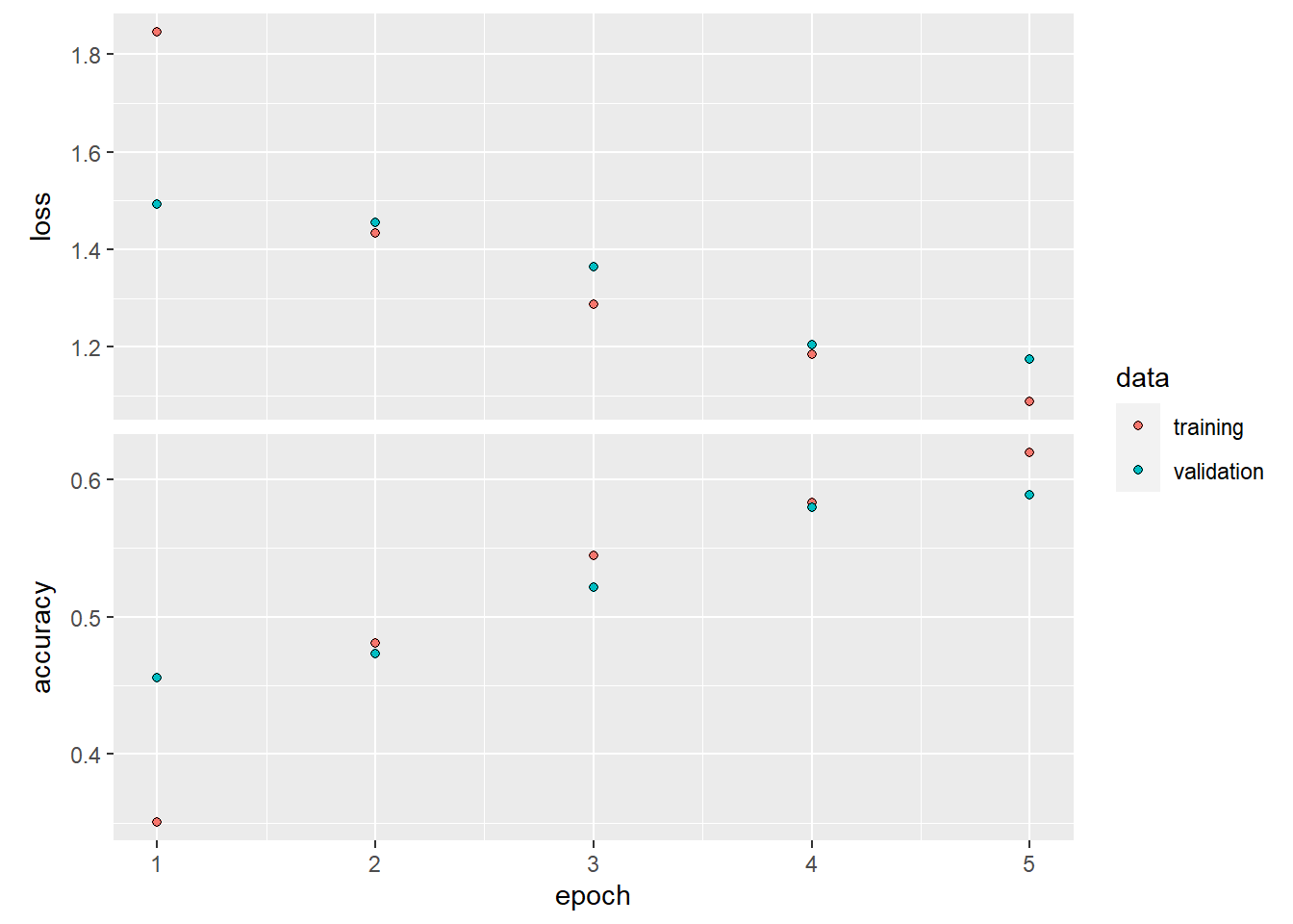
model %>% save_model_hdf5("D:/image/DeepLearning-ComputerVision/models/cats_and_dogs_small_1.h5")

We can plot the loss and accuracy of the model over the training and validation data during training. It shows an overfitting phenomenon. The training accuracy increases linearly over time wheras tha validation accuracy stops under a less important vale.

plot(history)

4.4.1.4 Data augmentation

Overfitting can be caused by the small quantity of samples for learning. Data augmentation consists of generating more training data from existing training samples by augmenting the samples via a number of random transformations that generates realistic and possible images. This helps in exposing the model to more aspects of the data and generalize better.

In keras, we can define a number of random trasformations on the images with image_data_generator

datagen = image_data_generator(
  rescale =  1/255,
  rotation_range = 40, # randomly rotate the pictures
  width_shift_range = 0.2, # a fraction of total width within which translate pictires horizontally
  height_shift_range = 0.2, # a fraction of total height within which translate pictires vertically
  shear_range = 0.2, # shifting image
  zoom_range = 0.2, # zooming inside the picture
  horizontal_flip = TRUE,
  fill_mode = "nearest"
)

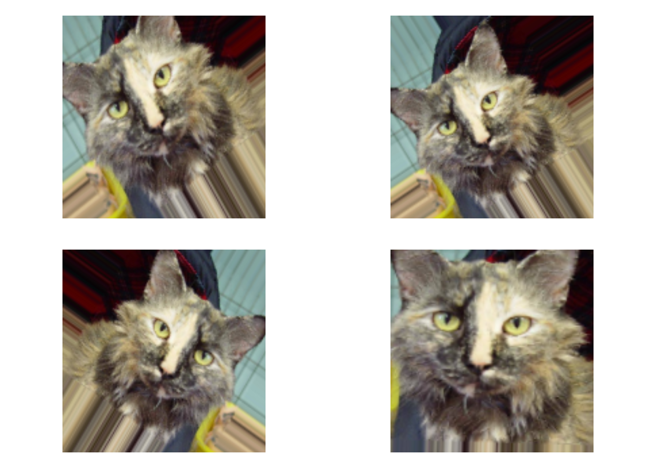
We can plot transformation effects one sample of image

# specify dir
train_cats_dir = "D:/image/DeepLearning-ComputerVision/data/cats_and_dogs_small/train/cats"
# load data
fnames = list.files(train_cats_dir, full.names = TRUE)
img_path = fnames[[2]] # choose one image to argument

img = image_load(img_path, target_size = c(150,150)) # read the image and resize it
img_array = image_to_array(img) # convert the image to an array of shape (150,150,3)
img_array = array_reshape(img_array, c(1,150,150,3)) # reshape the array

# generate batches of randomly transformed images
augmentation_generator = flow_images_from_data(
  img_array,
  generator = datagen,
  batch_size = 1
)

# plot the images
op = par(mfrow = c(2,2), pty = "s", mar = c(1,0,1,0))
for ( i in 1:4){
  batch = generator_next(augmentation_generator)
  plot(as.raster(batch[1,,,]))
}

par(op)

Now wa can train the network using data augmentation generator

# apply data augmentation generator to train
train_generator = flow_images_from_directory(
  train_dir,#traget directory
  datagen,# data generator
  target_size = c(150,150),
  batch_size = 32,
  class_mode = "binary"
)
# load test data
test_datagen = image_data_generator(rescale = 1/255)
# the validation data shouldn't be augmented
validation_generator = flow_images_from_directory(
  validation_dir,
  test_datagen,
  target_size = c(150,150),
  batch_size = 32,
  class_mode = "binary"
)
# fit the model
history = model %>% fit_generator(
  train_generator,
  steps_per_epoch = 100,
  epochs = 2,
  validation_data = validation_generator,
  validation_steps = 50
)

let’s save the model

model %>% save_model_hdf5("D:/image/DeepLearning-ComputerVision/models/cats_and_dogs_small_2.h5")

plot(history)

4.4.2 Dataset: CIFAR10

4.4.2.1 Download and prepare the CIFAR10 dataset

We will use CNN to classifiy CIFAR10 dataset which consists of 60,000 color images in 10 classes (6,000 images in each class). It contains 50,000 images for training and 10,000 images for testing.

library(tensorflow)

## 
## Attaching package: 'tensorflow'

## The following object is masked from 'package:caret':
## 
##     train

library(keras)
cifar = dataset_cifar10()
dim(cifar$train$x)

## [1] 50000    32    32     3

We can plot the first 25 images to verify the data:

cifar = dataset_cifar10()


class_names <- c('airplane', 'automobile', 'bird', 'cat', 'deer',
                 'dog', 'frog', 'horse', 'ship', 'truck')

index <- 1:30

par(mfcol = c(5,6), mar = rep(1, 4), oma = rep(0.2, 4))
cifar$train$x[index,,,] %>% 
  purrr::array_tree(1) %>%
  purrr::set_names(class_names[cifar$train$y[index] + 1]) %>% 
  purrr::map(as.raster, max = 255) %>%
  purrr::iwalk(~{plot(.x); title(.y)})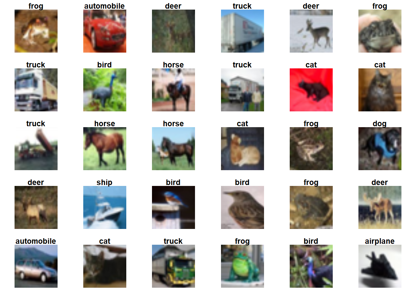

4.4.2.2 Build the model

We will build a convolution base for the model follwing a common pattern: a stck of Conv2D and MaxPooling2D layers. As input, a CNN takes tensors of shape (image_height, image_width, channels). The format of cifar images is (32,32,3).

model = keras_model_sequential() %>% 
  layer_conv_2d(filters = 32, kernel_size = c(3,3), activation = "relu", input_shape = c(32,32,3)) %>% 
  layer_max_pooling_2d(pool_size = c(2,2)) %>% 
  layer_conv_2d(filters = 64, kernel_size = c(3,3), activation = "relu") %>% 
  layer_max_pooling_2d(pool_size = c(2,2)) %>% 
  layer_conv_2d(filters = 64, kernel_size = c(3,3), activation = "relu")

summary(model)

## Model: "sequential_4"
## ________________________________________________________________________________
## Layer (type)                        Output Shape                    Param #     
## ================================================================================
## conv2d_7 (Conv2D)                   (None, 30, 30, 32)              896         
## ________________________________________________________________________________
## max_pooling2d_6 (MaxPooling2D)      (None, 15, 15, 32)              0           
## ________________________________________________________________________________
## conv2d_8 (Conv2D)                   (None, 13, 13, 64)              18496       
## ________________________________________________________________________________
## max_pooling2d_7 (MaxPooling2D)      (None, 6, 6, 64)                0           
## ________________________________________________________________________________
## conv2d_9 (Conv2D)                   (None, 4, 4, 64)                36928       
## ================================================================================
## Total params: 56,320
## Trainable params: 56,320
## Non-trainable params: 0
## ________________________________________________________________________________

We will add a dense layr on the top of our covolutional base. Dense layers take vectors as input (which are 1D). So, we need to flatten the 3D output of the convoltion base to 1D before adding layers on top. CIFAR data has 10 output classes, so the last layer need 10 outputs and a softmax activation.

model %>% 
  layer_flatten() %>% 
  layer_dense(units = 64, activation = "relu") %>% 
  layer_dense(units = 10, activation = "softmax")

summary(model)

## Model: "sequential_4"
## ________________________________________________________________________________
## Layer (type)                        Output Shape                    Param #     
## ================================================================================
## conv2d_7 (Conv2D)                   (None, 30, 30, 32)              896         
## ________________________________________________________________________________
## max_pooling2d_6 (MaxPooling2D)      (None, 15, 15, 32)              0           
## ________________________________________________________________________________
## conv2d_8 (Conv2D)                   (None, 13, 13, 64)              18496       
## ________________________________________________________________________________
## max_pooling2d_7 (MaxPooling2D)      (None, 6, 6, 64)                0           
## ________________________________________________________________________________
## conv2d_9 (Conv2D)                   (None, 4, 4, 64)                36928       
## ________________________________________________________________________________
## flatten_3 (Flatten)                 (None, 1024)                    0           
## ________________________________________________________________________________
## dense_12 (Dense)                    (None, 64)                      65600       
## ________________________________________________________________________________
## dense_13 (Dense)                    (None, 10)                      650         
## ================================================================================
## Total params: 122,570
## Trainable params: 122,570
## Non-trainable params: 0
## ________________________________________________________________________________

4.4.2.3 Compile and train the model

# launch TensorBoard (data won't show up until after the first epoch)
# tensorboard("logs/run_a")

model %>% compile(
  optimizer = "adam",
  loss = "sparse_categorical_crossentropy",
  metrics = "accuracy"
)

history <- model %>% 
  fit(
    x = cifar$train$x, y = cifar$train$y,
    epochs = 5,
    validation_data = unname(cifar$test),
    verbose = 2
    # callbacks = callback_tensorboard("logs/run_a")
  )

4.4.2.4 Evaluate the model

plot(history)

evaluate(model, cifar$test$x, cifar$test$y, verbose = 0)

## $loss
## [1] 1.175468
## 
## $accuracy
## [1] 0.5889