Chapter 3 Neural Networks
3.1 Structure of neural network
Training a neural network concerns these objects: layers, input data and corresponding targets, loss function and optimizer. The network is composed of layers stacked together, maps the input data to predictions. The loss function is used to compare the predictions to the targes and generats a loss value (difference between perdicted and expected values or classes). Then, an optimizer is used used to minimize the loss value by updating the network’s weights.
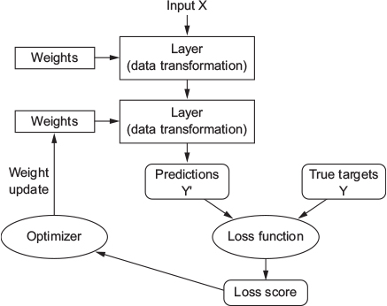
Neural network structure (source:https://livebook.manning.com/book/deep-learning-with-r/chapter-3/19)
3.1.1 Tensors
3.1.1.1 Dimensions
The fundamental data structure manipulated by neural networks is Tensors. Tensors are a generalization of vectors and matrices to an arbitrary number of dimensions (called axis).
- scalars (0D tensors): A tensor with only one number is called scalar
- Vectors (1D tensors): A tensor with one dimension is called vector.
## num [1:3] 1 2 3## [1] 3This vector has 3 possible values, so it is three-dimensional vector. This 3D vector has only one axis and 3 dimensions along its axis. In opposition to 3D tensor that has 3 axis, with any number of dimensions in each axis. Dimensionality can represent either the number of entries along a specific axis or the number of axes in a tensor.
- Matrices (2D tensors): A tensor with two axes (rows and columns).
##      [,1] [,2] [,3] [,4] [,5]
## [1,]    0    0    0    0    0
## [2,]    0    0    0    0    0
## [3,] 0 0 0 0 0## [1] 3 5- 3D and higher dimensions tensors: We can obtain a 2D tensor by packing matrices in a new array. The obtained object can be represented visually as a cube. By packing the 3D tensors in an array we obtain a 4D tensor and so on.
## num [1:2, 1:3, 1:2] 0 0 0 0 0 0 0 0 0 0 ...## [1] 2 3 23.1.1.2 Properties
A tensor is defined by three main prperties:
- Number of axis: For example, a 3D tensor has 3 axis
- Shape: It is an integer vector that denotes the number of dimensions the tensor has along each axis. For example, a matriw with 3 rows and 5 columns is a tensor with the shape
(3,5). - Data type: The type o data stored in the tensor: integer, double, character…
Let’s present an example with the mnist dataset
Now we display the properties the tensor train_images
## [1] 3## [1] 60000 28 28## [1] "integer"So we have a 3D tensor of integer. It is an array of 60,000 matrices of 28x28 integers. Let’s plot one matrix

3.1.1.3 Data batches
In deep-learning models we don’t process the whole dataset at once, but we break it into small batches. It consists of slicing the samples dimension. For example we will take a batch of MNIST digits of size 128:
3.1.1.4 Examples of data tensors
- Vector data They are 2D tensors of shape
(samples, features) - Timeseries and sequence data They are 3D tensors of shape
(samples, timesteps, features) - Image data They are 4D tensors of shape
(samples, height, width, channels) - Video data They are 5D tensors of shape
(samples,frames, channels, height, width)
3.1.1.5 Tensors operations
https://livebook.manning.com/book/deep-learning-with-r/chapter-2/244
3.1.2 Layers
The layers cnsists on data-processing modules that take as input one or more tensors and generates as outputs one or more tensors. The layers conrain the learned weights taht represent the network’s knowledge. The layers’ types depend on the data types used as input:
- Densly connecte (fully connected) layers: they are used for
vectordata taht are stored in 2D tensors of shape(samples, features) - Recurrent layers: they are used for
sequencedata that are stred in 3D tensors of shapesamples, timsteps, features - Convolution layers: they are used for
ìmagedata, taht are stored in 4D tensors
Building deep-learning model in Keras is done by stacking compatible layers together. To respect layer compatibilty, every layer only accept input tensors with a specific shape.
In this example, we are creating a layer that only accept as input 2D tensors where the first dimension is 784. This layer will return a tensor where the first dimension has been transformed to be 32. Then, this layer can only be connected to a layer taht expects as 32-dimensional vector as input. In keras, the layers we add to our models are automatically built to match the shape of the incoming mayer.
model = keras_model_sequential() %>%
  layer_dense(units = 32, input_shape = c(784)) %>%
  layer_dense(units = 32)
SO here we didn’t specify the input shape of the second layer. It was automatically inferred based on the shape of the previous layer (32).
3.1.3 Activation functions
- Rectified linear unit (ReLU)
- Sigmoid
- Softmax
3.1.4 Loss functions and optimizers
Once the network layers architectue is defined, we have specify two elements:
- loss function: It represents the quantity that we want to minimize during the training phase.
- Optimizer: It represnts the method used by the network to update the weight based on loss function. It consists on implementing a specific variant of stochastic graient descent optimization.
We can have a network with multiple loss funtions (when the network ghave multiple outpus). Since the gradient-descent process need to be based on a sigle loss value, all loasses values have to be combined i a single measure (by averaging for example).
It is important to select the appropriate loss function depending in the learning problem. There are some guidlines we can follow for common situations:
- We use binary crossentropy for a Two-class classification problem
- We use categorical crossentropy for a Two-class classification problem
- we use the mean-squared error for a regression problem
3.1.5 Building a Neural Network from scratch
##      [,1] [,2] [,3] [,4]
## [1,]    1    0    1    0
## [2,]    1    0    1    1
## [3,] 0 1 0 1## [,1]
## [1,] 1
## [2,] 1
## [3,] 0#sigmoid function
sigmoid<-function(x){
1/(1+exp(-x))
}
# derivative of sigmoid function
derivatives_sigmoid<-function(x){
x*(1-x)
}
# variable initialization
epoch=1000
lr=0.1
inputlayer_neurons=ncol(X)
hiddenlayer_neurons=3
output_neurons=1
#weight and bias initialization
wh=matrix( rnorm(inputlayer_neurons*hiddenlayer_neurons,mean=0,sd=1), inputlayer_neurons, hiddenlayer_neurons)
bias_in=runif(hiddenlayer_neurons)
bias_in_temp=rep(bias_in, nrow(X))
bh=matrix(bias_in_temp, nrow = nrow(X), byrow = FALSE)
wout=matrix( rnorm(hiddenlayer_neurons*output_neurons,mean=0,sd=1), hiddenlayer_neurons, output_neurons)
bias_out=runif(output_neurons)
bias_out_temp=rep(bias_out,nrow(X))
bout=matrix(bias_out_temp,nrow = nrow(X),byrow = FALSE)
# forward propagation
for(i in 1:epoch){
hidden_layer_input1= X%*%wh
hidden_layer_input=hidden_layer_input1+bh
hidden_layer_activations=sigmoid(hidden_layer_input)
output_layer_input1=hidden_layer_activations%*%wout
output_layer_input=output_layer_input1+bout
output= sigmoid(output_layer_input)
# Back Propagation
E=Y-output
slope_output_layer=derivatives_sigmoid(output)
slope_hidden_layer=derivatives_sigmoid(hidden_layer_activations)
d_output=E*slope_output_layer
Error_at_hidden_layer=d_output%*%t(wout)
d_hiddenlayer=Error_at_hidden_layer*slope_hidden_layer
wout= wout + (t(hidden_layer_activations)%*%d_output)*lr
bout= bout+rowSums(d_output)*lr
wh = wh +(t(X)%*%d_hiddenlayer)*lr
bh = bh + rowSums(d_hiddenlayer)*lr
}
output## [,1]
## [1,] 0.95657617
## [2,] 0.94810285
## [3,] 0.081490643.2 Introduction to Keras
Keras is library for developing deep learning models. It dosen’t handle low-level operations such as tensor manipulation. But it relies on specialized tensor libraries as backend engine such as TensorFlown Theano and Mirosoft Cognitive Toolkit (CNTK). Via TensorFlow, Keras is able to run on both CPUs and GPUs. When running on CPU, TensorFlow is itself wrapping a low-lvel library for tensor operations called Eigen. On GPU, TensorFlow wraps a library called NIVIDIA CUDA Neural Network library (cuDNN).
3.2.1 Installing keras
# Installing keras package
install.packages("keras")
# Install the core keras library and TensorFlow
library(keras)
install_keras()
This installation provide us with a default CPU-based installation of keras and TensoFlow. If we wan to train our models on a GPU and we have properly configured CUDA and cuDNN libraries, we can install the GPU-based version of TensroFlow backend engine as follows:
3.2.2 building model with keras
Here is a typical keras workflow:
- Define training data: iput tensors and target tensors
- Define a network of layers that maps the inputs to the targets
model = keras_model_sequential() %>%
  layer_dense(units = 32, input_shape = c(784)) %>%
layer_dense(units = 10, activation = "softmax")- Specify the learning process by defining a losss function, an optimizer, and some metrics to monitor
model %>% compile(
  optimizer = optimizer_rmsprop(lr = 0.0001),
  loss = "mse",
  metrics = c("accuracy")
)- Iterate on the training data using the
fit()method of our model
3.2.3 The Kears Functional API
The common configuration of keras models is based on sequential layer stacking keras_model_sequential. However, in some applications we may need to develop models with multiple inputs, multiple outputs and more complex interactions between layers. These make these model look lik graphs.
Example of multi-inputs: let’s imagine we are facing to a learning problem based on text ad image data (for example predicting item prices based on text description and pictures). We can propose two seperate models and average the prediction outputs at the end. Another way consists on jointly learn a more accurate model based on both text and image inputs.
Example of multi-outpus: let’s imagine we have some text corpus and we want to predict both the type (romance vs thriller classification) and the date when it was written. We can train two sperate models: a classifier for text types and a regressor for date prediction. But since these properties may be dependents and correlated, it would be more accurate to build a odel that jointly learn to predict types and date.
Example of complex architectures: Many recent networks architecture require complex connexions between layers or group of layers: The Inception family of CNN process several parallel convolutional branches whose outputs are merged back into a single tensor, the ResNet family add residual connections that consists of reinjecting past output tensor to later output tensor in order to prevent inofmation loss along the data processing flow.
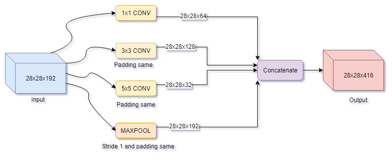
Inception module (source: https://www.oreilly.com/library/view/hands-on-convolutional-neural/9781789130331/41617ecf-cd1e-467c-93d9-ecf265979317.xhtml)
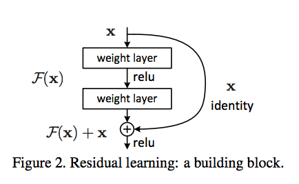
Residual connections (source: https://towardsdatascience.com/introduction-to-resnets-c0a830a288a4)
Here is how to define an equivalent to sequential model but using the functional API in a graph like model.
library(keras)
# sequential model
seq_model = keras_model_sequential() %>%
  layer_dense(units = 72, activation = "relu", input_shape = (64)) %>%
  layer_dense(units = 32, activation = "relu") %>%
  layer_dense(units = 10, activation = "softmax")
# equivalent functional model
input_tensor = layer_input(shape = c(64))
output_tensor = input_tensor %>%
  layer_dense(units = 32, activation = "relu") %>%
  layer_dense(units = 32, activation = "relu") %>%
  layer_dense(units = 10, activation = "softmax")
model = keras_model(input_tensor,output_tensor)
model
## Model
## Model: "model"
## ________________________________________________________________________________
## Layer (type) Output Shape Param #
## ================================================================================
## input_1 (InputLayer) [(None, 64)] 0
## ________________________________________________________________________________
## dense_3 (Dense) (None, 32) 2080
## ________________________________________________________________________________
## dense_4 (Dense) (None, 32) 1056
## ________________________________________________________________________________
## dense_5 (Dense) (None, 10) 330
## ================================================================================
## Total params: 3,466
## Trainable params: 3,466
## Non-trainable params: 0
## ________________________________________________________________________________3.2.4 Models as Directed acyclic graphs of layers
With the functional API, we can build models with complex architecture. Keras provides the possibility of modeling layers as direcetd acyclic graphs. It can be used for building models with inception like topology
branch_a = input %>% layer_conv2d(filters = 128, kernel_size = 1, activation = "relu", strides = 2)

branch_b = input %>%
  layer_conv2d(filters = 128, kernel_size = 1, activation = "relu") %>%
  layer_conv2d(filters = 128, kernel_size = 3, activation = "relu", strides = 2)

branch_c = input %>%
  layer_average_pooling_2d(pool_size = 3, strides = 2) %>%
  layer_conv2d(filters = 128, kernel_size = 3, activation = "relu")

branch_d = input %>%
  layer_conv2d(filters = 128, kernel_size = 1, activation = "relu") %>%
  layer_conv2d(filters = 128, kernel_size = 3, activation = "relu") %>%
  layer_conv2d(filters = 128, kernel_size = 3, activation = "relu", strides = 2)

output = layer_concatenate(list(branch_a, branch_b, branch_c, branch_d))
3.3 Monitoring deep learning models
3.3.1 Using callbacks
A callback is an object integrated to the model in the fit operation and is caled at different points durinf training phase. The callback object has access toall information about the state of the model and its performance. It can also act during the training for:
- Model checkpointing: saving the current weights of the mode at different points during the training
- Early stopping: Interrupting training when the validation loss is no longer improving and saving the best model obtained during training
- Dynamically adjusting the value of certain parameters during training such as the learning rate and the optimizer
- Logging training and validation metrics
Keras provides some built-in callbacks:
callback_model_checkpoint()
callback_early_stopping()
callback_learning_rate_scheduler()
callback_reduce_lr_on_plateau()
callback_csv_logger()
We can use callback_early_stopping to interrupt training once a target monitored metric gas stopped improving during some epochs. This type of callback can be used to stop training when the model starts overfitting. This callback is used in simultaneously with callback_model_checkpoint that enables saving continually the model during the training phase. We can also choose to save the optimal version of the model: the version that ends with best performance at the end of an epoch.
callbacks_list = list(
  # stop training when no improvement
  callback_early_stopping(
    # monitor accuracy metric
    monitor = "acc",
    # Stop training when accuracy has stopped improving for more than one epoch
    patience = 1
  ),
  # saving the current weights after every epoch
  callback_model_checkpoint(
    filepath = "my_model.h5",
    # we avoide overwriting the model file unless val_loss has improved. We keen the best model seen during training.
    monitor = "val_loss",
    save_best_only = TRUE
  )
)

model %>%  compile(
  optimizer = "rmsprop",
  loss = "binary_crossentropy",
  metrics = c("acc")
)

model %>% fit(
  x, y,
  epochs = 10,
  batch_size = 32,
  callbacks = callbacks_list,
  # because the callback ill monitor the validation loss, we ned to pass validation_data to the call to fit
  validation_data = list(x_val, y_val)
)
The ‘callbacks’ can be used for reducing the learning rate once validation loss has stopped improving. reducing or increasing the learning rate in case of loss plateau is consiedered as an effective strategy to get out of local minima dring training.
callbacks_list = list(
  callback_reduce_lr_on_plateau(
    # monitor the model validation loss
    monitor = "val_loss",
    # dividing the learning rate by 10 when triggered
    factor = 0.1,
    # the callback is triggered after the validation loss has stopped improving for 10 epochs
    patience = 10
  )
)

model %>% fit(
  x, y,
  epochs = 10,
  batch_size = 32,
  callbacks = callbacks_list,
  # because the callback ill monitor the validation loss, we ned to pass validation_data to the call to fit
  validation_data = list(x_val, y_val)
)
3.3.2 TensorBoard
TensorBoard is a browser-based visualization tool packaged with TensorFlow. It helps to visually montor mterics during training, show model architecture, visalize histograms and activations and gradients…
Here is an example of using TensorBoard fo IMDB sentiment-analysis application.
# limiing the number of words to consider as features for this example
max_features = 2000
# cut text in 500 words for this example
max_len = 500
# load data
imdb = dataset_imdb(num_words = max_features)
# split train and test
c(c(x_train, y_train),c(x_test, y_test)) %<-% imdb
# pad sequences
x_train = pad_sequences(x_train, maxlen = max_len)
x_test = pad_sequences(x_test, maxlen = max_len)
# build model
model = keras_model_sequential() %>%
  layer_embedding(input_dim = max_features, output_dim = 128, input_length = max_len, name = "embed") %>%
  layer_conv_1d(filters = 32, kernel_size = 7, activation = "relu") %>%
  layer_max_pooling_1d(pool_size = 5) %>%
  layer_conv_1d(filters = 32, kernel_size = 7, activation = "relu") %>%
  layer_global_max_pooling_1d() %>%
  layer_dense(units = 1)
summary(model)
# compile model
model %>%  compile(
  optimizer = "rmsprop",
  loss = "binary_crossentropy",
  metrics = c("acc")
)
We create a directory where we can store the log files generated
# lunch tensorboard
tensorboard("log_directory")

# define callbacks
callbacks = list(
  callback_tensorboard(
    log_dir = "log_directory",
    # record activation histograms every 1 epoch
    histogram_freq = 1,
    # record embedding data every 1 epoch
    embeddings_freq = 1,
  )
)

# fit the model
history = model %>%  fit(
  x_train, y_train,
  epochs = 5,
  batch_size = 128,
  validation_split = 0.2,
  calbacks = callbacks
)
3.4 Batch normalization
Batch normalization helps mdels learn and generalize better on new data. The most common methods for batch normalization consists of centering the data on zero by substracting the mean from the data and changing standard deviation of data to 1 by dif=viding the data by ots standard deviation.
mean = apply(train_data, 2, mean)
std = apply(train_data, 2, sd)
train_data = scale(train_data, center = mean, scale = std)
test_data = scale(test_data, center = mean, scale = std)
Batch normalization should be implemented after every transofmation operated by the network. In keras, it is represenred as a specific layer: layer_batch_normalization. It is commonly used after a convolution or densly connected layers:
3.5 Overfitting handling
3.5.1 Reducing the network’s size
The simplest way to avoid overfitting is to reduce the size of the model: the number of learnable parameters whiwh are dependant on the number of layers and the number of units by layer.
3.5.2 Adding weight regularization
The weight regularizaion technics is based on the hypothesis that a simple model, with fewer parametrs or where the distribution of parameter values has less entropy, may behave better with new unseed data. Tehrefore, we can avoid overfitting by adding constraints in the model and forcing its weights to take only small values. This makes the distribution of weight vales more regular. This technic is called weight regularization. It is implemented by adding to the loss function of the netork a cost associated with having large weights. We can define the cost in two ays:
- L1 regularization: The cost added is propotional to the absolute value of the weight coefficients
- L2 regularization (weight decay): The cost added is propotional to the square of the value of the weight coefficients
model = keras_model_sequential() %>%
  layer_dense(units = 16, kernel_regularizer = regularizer_l2(0.001),
              activation = "relu", input_shape = c(10000)) %>%
  layer_dense(units = 16, kernel_regularizer = regularizer_l2(0.001),
              activation = "relu", input_shape = c(10000)) %>%
  layer_dense(units = 1, activation = "sigmoid")
regularizer_l2(0.001) means that every coefficien in the weight matrix of the layer will add 0.001*weight_coefficient_value to the total loss of the network.
Since the penality is only added at training phase, the loss at the training phase will be much higher thatn the loss in the test phase.
3.5.3 Adding dropout
Dropout consists on randomly setting to zero a number of output features of a layer during the training.
The idea behind dropout technic is to introduce noise in the output values of a layer in order to remove non significant features.
The dropout rate is the fraction of the features that are set to zero. It is usually between 0.2 and 0.5.
During the test phase, no units are dopped out but the layer’s output values are scaled down by a factor equal to the dropout rate to have same number of units active.
We can implement the both operations at training phase in order to have unchanged output at test phase. Therefore, we scale up by the dropout rate rather than scaling down.
layer_dropout = layer_dropout * sample(0:1, length(layer_output), replace = TRUE)
layer_dropout = layer_dropout / 0.5
let’s see how to add dropout in our model with keras