Chapter 3 Word embeddings

This section is based on this book: https://github.com/jjallaire/deep-learning-with-r-notebooks

3.1 Vectorizing text

It is the process of transforming text into numeric tensors. It consists of applying some tokenization scheme and then associating numeric vectors with the generated tokens. The generated vectos are packed into sequence tensors and fed into deep neural network. There are different ways to associate a vector within a token such as one-hot encoding and token embedding (typically used for words and called word embedding).

3.2 One-hot encoding

It consists of one-hot encoding the words existing in a sentence based on the whole vocabulary.We create a vector with length equal to the vocabulary and we place a one in the index that corresponds to the word existing in the sentences. Then, we can concatenate the one-hot vectors for each word. This method is considered as inefficient since we obtain a sparse one-hot encoded vector (most indices are zero).

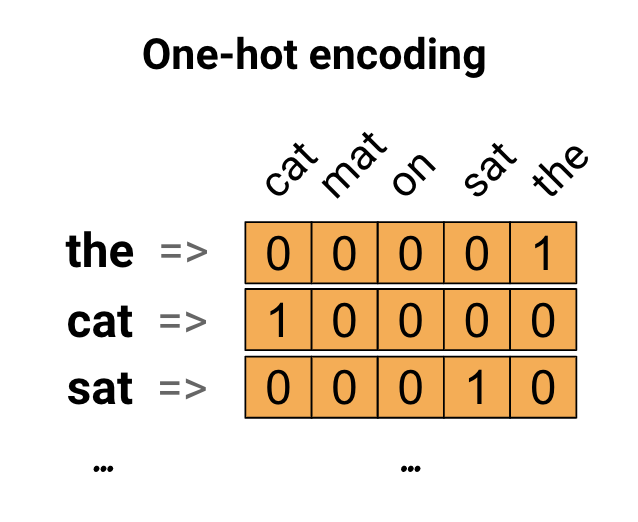
One-hot encoding (source:https://www.tensorflow.org/tutorials/text/word_embeddings)

library(keras)
samples <- c("The cat sat on the mat.", "The dog ate my homework.")
# Creates a tokenizer, configured to only take into account the 1,000 
# most common words, then builds the word index.
tokenizer <- text_tokenizer(num_words = 1000) %>%
  fit_text_tokenizer(samples)
# Turns strings into lists of integer indices
sequences <- texts_to_sequences(tokenizer, samples)
# You could also directly get the one-hot binary representations. Vectorization 
# modes other than one-hot encoding are supported by this tokenizer.
one_hot_results <- texts_to_matrix(tokenizer, samples, mode = "binary")
# How you can recover the word index that was computed
word_index <- tokenizer$word_index
cat("Found", length(word_index), "unique tokens.\n")

## Found 9 unique tokens.

3.3 Word embeddings methods

The vectors obtained with one-hot encoding are binary, sparse and very high dimensional (same dimensionality of the number of words in the vocabulary). However, “word embeddings” are low-dimensional dense vectors (as oposite to sparse vectors). They are learned from data. They are commonly 256-dimensional, 512 dimensiona, or 1024-dimensional when dealing with large vocabularies.

There are two methods for obtaining word embedings:

• Learn word embeddings jointly with a specified task (document classification, sentimenta alnaysis…). For this, we start with random word vectors and learn the word vectors in the same way that we learn the weights of a neural network.
• Use a “pre-trained” word embeddings and apply it to our specific task

3.3.1 Learn world embeddings

Word embeddings aim t mapping human language into a geometric space in a way that geometric relationships between word vectors reflect the semantic relationships netween the words. For example, synonyms should be embedded into similar word vectors. We expect that geometric distance between any two word vectors represent semantic distance of the associated words. We can site among common meaningful geometric transformations in word embeddings the “gender vectors” and “plural vectors”. For example, by adding a “female vector” to the vector “king”, we obtain the vector “queen”. In the same way, by adding a “plural vector”, we obtain “kings”. It is hard to find the “ideal” word embedding space to perfectly map general human language. Word embedding performance depends on the task we are working on. A word embedding for Ensglish-language movie review sentiment analysis model may look very different from an English-language legal document classification model since the importance of some semantic relationships varies from task to task. Therefore, it is useful to learn a new embedding space with every new task. Keras offers the possibility of learning embeddings using layer_embedding().

# the embedding layer takes at least two arguments:
# - the number of posssible tokens, here 1000
# - the dimensionality of the embeddings, here 64
embedding_layer = layer_embedding(input_dim = 1000, output_dim = 64)

The embedding_layer is like a dictionary that maps integer indices to dense vectors. It takes as input a 2D tensor of integers, of shape (samples, sequence_length), where each entry is a sequence of integers. It generates a 3D floating-point tensor, of shape (samples, sequence_length, embedding_dimensionality.

Let’s apply embedding_layer to the IMDB movie-review sentiment prediction task. We will consider only the top 10,000 most common words and cut off the review after only 20 words. The network will learn 8-dimensional embeddings for each of the 10,000 words, turn the input integer sequences (2D integer tensor) into embedded sequences (3D float tensor), flatten the tensor to 2D, and train a single dense layer on top for classification.

library(keras)
# Number of words to consider as features
max_features = 10000
# cut texts after this number of words (among top max_features most common words)
maxlen = 20
# load the data as lists of integers
imdb = dataset_imdb(num_words = max_features)
c(c(x_train, y_train), c(x_test, y_test)) %<-% imdb
# This turns our lists of integers
# into a 2D integer tensor of shape `(samples, maxlen)`
x_train = pad_sequences(x_train, maxlen = maxlen)
x_test = pad_sequences(x_test, maxlen = maxlen)

library(keras)
model = keras_model_sequential() %>% 
  # we specify the maxmum input length to our embedding layer
  # so we can later flatten the embedded inputs
  layer_embedding(input_dim = 10000, output_dim = 8, input_length = maxlen) %>% 
  # we flatten the 3D tensor of embeddings into a 2D tensor of shape (samples, maxlen * 8)
  layer_flatten() %>% 
  # We add the classifier on top 
  layer_dense(units = 1, activation = "sigmoid")

model %>%  compile(
  optimizer = "rmsprop",
  loss = "binary_crossentropy",
  metrics = c("acc")
)

history = model %>%  fit(
  x_train, y_train,
  epochs = 10, #10
  batch_size = 32,
  validation_split = 0.2
)

plot(history)

## `geom_smooth()` using formula 'y ~ x'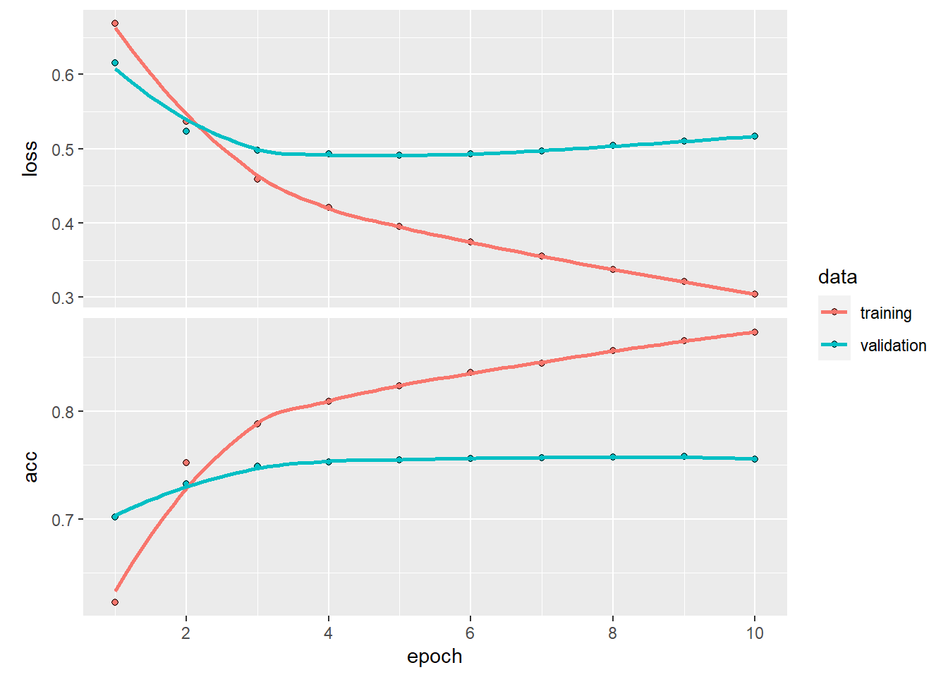

3.3.2 Pre-trained word embeddings

When we have little training data available to learn task-specific word embedding base on our vocabulary, it is preferable to use a pre-trained word embeddings. This technic is simular to transfer learning in image classification tasks, where we use a pretrained classifier. A pre-computed embedding is supposed to capture generic aspects of language structure. These word embeddings are trained based on co-occurence of words in sentences and documents within a large corpus of text. We can distinguish two main powerful word embeddings models: Word2Vec and GloVe.

3.3.2.1 Word2Vec

3.3.2.2 Glove

3.4 Applications

3.4.1 Using Skip-Gram

We use the Amazon Fine Foods Reviews datset which consists of 500,000 reviews of Amazon fine food including product and user information, ratings, and narrative text. source: https://blogs.rstudio.com/tensorflow/posts/2017-12-22-word-embeddings-with-keras/

3.4.1.1 Getting the data

# we download the data
download.file("https://snap.stanford.edu/data/finefoods.txt.gz", "finefoods.txt.gz")

Now we load the plain text reviexs:

library(readr)
library(stringr)
reviews <- read_lines("finefoods.txt.gz") 
reviews <- reviews[str_sub(reviews, 1, 12) == "review/text:"]
reviews <- str_sub(reviews, start = 14)
reviews <- iconv(reviews, to = "UTF-8")
head(reviews, 2)

## [1] "I have bought several of the Vitality canned dog food products and have found them all to be of good quality. The product looks more like a stew than a processed meat and it smells better. My Labrador is finicky and she appreciates this product better than  most."
## [2] "Product arrived labeled as Jumbo Salted Peanuts...the peanuts were actually small sized unsalted. Not sure if this was an error or if the vendor intended to represent the product as \"Jumbo\"."

3.4.1.2 Preprocessing

We use text_tokenizer in order to transform each review into a sequence of integer tokens. By fixing num_words = 20000, we assign integer token to each of the 20,000 most common words (the other words will be assigned to token 0).

library(keras)
tokenizer = text_tokenizer(num_words = 20000)
tokenizer %>% fit_text_tokenizer(reviews)
#we can show the number of documents
tokenizer$document_count

## [1] 568454

# we can show the word index list
tokenizer$word_index %>%
  head()

## $the
## [1] 1
## 
## $i
## [1] 2
## 
## $and
## [1] 3
## 
## $a
## [1] 4
## 
## $to
## [1] 5
## 
## $it
## [1] 6

3.4.1.3 Skpi-Gram model

In the skip-gram model, we use each word as input to a log-linear classifier, then predict words within a certain range before and after this word. It would be very compyationally expensive if we outpt a probability distribution over all the vocabulary for each target word we input in the model. Therefore, we will use negative sampling. It consists of sampling some words that don’t appear i the context and train a binary classifier to predict if the context word we passed is truly from the context or not.

Let’s defin a generator function to yield batches for model training. This genratire function will receive a vector of texts, a tokenizer and the arguments for the skip-gram (the size of the window around each target word we exaine and how manu=y negative samples we ant to sample for each target word).

library(reticulate)
library(purrr)
skipgrams_generator <- function(text, tokenizer, window_size, negative_samples) {
  gen <- texts_to_sequences_generator(tokenizer, sample(text))
  function() {
    skip <- generator_next(gen) %>%
      skipgrams(
        vocabulary_size = tokenizer$num_words, 
        window_size = window_size, 
        negative_samples = 1
      )
    x <- transpose(skip$couples) %>% map(. %>% unlist %>% as.matrix(ncol = 1))
    y <- skip$labels %>% as.matrix(ncol = 1)
    list(x, y)
  }
} 

We define now the keras model using kers functional API.

# Dimension of the embedding vector
embedding_size = 128 
# how many words to consider left and right
skip_window = 5
# number of negative examples to sample for each word
num_sampled = 1

We will write placeholders for the inputs using layer_input function

input_target = layer_input(shape = 1)
input_context = layer_input(shape = 1)

Now let’s define the embedding matrix. The embedding is a matrix with dimensions (vocabulary, embedding_size) that acts as lookup table for the word vectors.

embedding <- layer_embedding(
  input_dim = tokenizer$num_words + 1, 
  output_dim = embedding_size, 
  input_length = 1, 
  name = "embedding"
)

target_vector <- input_target %>% 
  embedding() %>% 
  layer_flatten()

context_vector <- input_context %>%
  embedding() %>%
  layer_flatten()

Now we define how the target_vector will be related to the context_vector in order to make the network output equal to 1 when the context word really appeared in the contexte and 0 otherwise. We want target_vector to be similar to the context_vector if they appeared in the same context. A typical measure of similarity is the cosine similarity. Give two vectors A and B the cosine similarity is defined by the Euclidean Dot product of A and B normalized by their magnitude. As we don’t need the similarity to be normalized inside the network, we will only calculate the dot product and then output a dense layer with sigmoid activation.

dot_product <- layer_dot(list(target_vector, context_vector), axes = 1)
output <- layer_dense(dot_product, units = 1, activation = "sigmoid")

Let’s create and compile the model

model <- keras_model(list(input_target, input_context), output)
model %>% compile(loss = "binary_crossentropy", optimizer = "adam")
summary(model)

## Model: "model"
## ________________________________________________________________________________
## Layer (type)              Output Shape      Param #  Connected to               
## ================================================================================
## input_1 (InputLayer)      [(None, 1)]       0                                   
## ________________________________________________________________________________
## input_2 (InputLayer)      [(None, 1)]       0                                   
## ________________________________________________________________________________
## embedding (Embedding)     (None, 1, 128)    2560128  input_1[0][0]              
##                                                      input_2[0][0]              
## ________________________________________________________________________________
## flatten_1 (Flatten)       (None, 128)       0        embedding[0][0]            
## ________________________________________________________________________________
## flatten_2 (Flatten)       (None, 128)       0        embedding[1][0]            
## ________________________________________________________________________________
## dot (Dot)                 (None, 1)         0        flatten_1[0][0]            
##                                                      flatten_2[0][0]            
## ________________________________________________________________________________
## dense_1 (Dense)           (None, 1)         2        dot[0][0]                  
## ================================================================================
## Total params: 2,560,130
## Trainable params: 2,560,130
## Non-trainable params: 0
## ________________________________________________________________________________

3.4.1.4 Model training

To fit the model we need to specify the number of training steps and the number of epochs. We will use only one epoch for time computation reasons.

model %>%
  fit_generator(
    skipgrams_generator(reviews, tokenizer, skip_window, negative_samples), 
    steps_per_epoch = 2000, epochs = 2
  )

We can extract the embedding matrix from the model using the get_weights() function.

library(dplyr)

embedding_matrix <- get_weights(model)[[1]]

words <- data_frame(
  word = names(tokenizer$word_index), 
  id = as.integer(unlist(tokenizer$word_index))
)

## Warning: `data_frame()` is deprecated as of tibble 1.1.0.
## Please use `tibble()` instead.
## This warning is displayed once every 8 hours.
## Call `lifecycle::last_warnings()` to see where this warning was generated.

words <- words %>%
  filter(id <= tokenizer$num_words) %>%
  arrange(id)

row.names(embedding_matrix) <- c("UNK", words$word)
dim(embedding_matrix)

## [1] 20001   128

head(embedding_matrix)

##          [,1]         [,2]        [,3]         [,4]        [,5]        [,6]
## UNK 0.0170815 -0.001318716  0.04716846 0.0001694448 -0.01495628  0.01284777
## the 0.1174329 -0.383204609 -0.14486948 0.2978044450  0.17878745 -0.28364837
## i   0.1669428 -0.247277036 -0.21312974 0.3762883544  0.28889671 -0.30660424
## and 0.1605144 -0.230475992 -0.17357136 0.3322810829  0.20980199 -0.25617325
## a   0.1201052 -0.146714032 -0.15440495 0.3936571181  0.22841439 -0.16955599
## to  0.1918591 -0.273127079 -0.17826691 0.3529382646  0.28203753 -0.24766697
##             [,7]        [,8]        [,9]       [,10]         [,11]
## UNK -0.007465005 -0.01517171  0.03539601  0.04036165 -0.0001689792
## the  0.299164832 -0.30537584 -0.36950541 -0.28876448 -0.2681583762
## i    0.362938732 -0.26686862 -0.34998602 -0.23723570 -0.2789547443
## and  0.310600638 -0.21819803 -0.34236768 -0.32119495 -0.1779417843
## a    0.278418452 -0.25963432 -0.35211003 -0.31251714 -0.2506726086
## to   0.347074360 -0.16523284 -0.32140639 -0.28436336 -0.2654981911
##             [,12]       [,13]      [,14]       [,15]       [,16]       [,17]
## UNK -0.0004024878 -0.01031651 -0.0329108 -0.03570246 -0.01811307 -0.02383759
## the  0.2796629667  0.31438842 -0.2472963  0.20960861 -0.28063810  0.17194803
## i    0.3474592566  0.33163065 -0.3115005  0.29770941 -0.32637006  0.09885775
## and  0.3099879324  0.28850329 -0.2122750  0.25450185 -0.35340777  0.15842982
## a    0.3022259772  0.33895627 -0.2288224  0.27653986 -0.23382780  0.15667632
## to   0.3335136473  0.27410549 -0.3449964  0.31313083 -0.33614126  0.02599920
##           [,18]       [,19]       [,20]       [,21]       [,22]       [,23]
## UNK 0.001930606 -0.04853332  0.03184437 -0.03507299  0.03099043 -0.01559343
## the 0.249449074  0.38885596 -0.10571286  0.03303542 -0.01977662  0.12713103
## i   0.266584009  0.32550138 -0.14738728  0.10654508  0.04477475  0.28375289
## and 0.281591505  0.33543691 -0.12878042  0.19387311  0.08222436  0.23661953
## a   0.213139340  0.28658631 -0.13082723  0.11910986  0.03216605  0.19973753
## to  0.144440114  0.35665330 -0.12372198  0.12668315  0.19030270  0.19488603
##           [,24]       [,25]       [,26]       [,27]       [,28]       [,29]
## UNK -0.02061616  0.01281368 -0.03231498 0.007334851  0.03719245  0.03511449
## the -0.17688274 -0.32929045 -0.29310527 0.289794803  0.13527869 -0.27275386
## i   -0.23470533 -0.32637039 -0.26748180 0.318160236  0.03208359 -0.21226105
## and -0.25599492 -0.34276465 -0.33586788 0.217786700  0.02351790 -0.27456364
## a   -0.17987984 -0.37211826 -0.33599785 0.294163078 -0.06172014 -0.27303630
## to  -0.25984651 -0.32187936 -0.29270798 0.297974795 -0.07057865 -0.25982314
##           [,30]         [,31]       [,32]        [,33]       [,34]       [,35]
## UNK -0.01691567  0.0008091219 -0.03200240 -0.006604362 -0.03469641 -0.03299238
## the  0.25344208  0.1719853282  0.07652652 -0.321915329  0.23948634  0.01470774
## i    0.22992177  0.0279782731  0.08346167 -0.304561466  0.12635729  0.02191944
## and  0.18178248  0.1102448180  0.08257330 -0.269136578  0.20793088 -0.09406497
## a    0.18358734  0.2180162519  0.05090325 -0.267941982  0.16697714  0.03600145
## to   0.25895324 -0.0176757276  0.13935305 -0.208568946  0.19998248 -0.05754858
##           [,36]      [,37]       [,38]       [,39]      [,40]        [,41]
## UNK  0.03315267 0.04222684 -0.02326957 -0.03361871 -0.0365397 -0.043440260
## the -0.28853074 0.37395093  0.20946701  0.15802002  0.2907013 -0.010865721
## i   -0.36051789 0.36837849  0.31315809  0.19938451  0.2936096 -0.131256387
## and -0.27480209 0.37666577  0.28615251  0.18097939  0.2794661 -0.006140751
## a   -0.27293894 0.33773720  0.32223794  0.22417280  0.2404891 -0.039677981
## to  -0.30174917 0.30440938  0.29927579  0.14390787  0.2480671 -0.093178861
##          [,42]       [,43]     [,44]       [,45]      [,46]       [,47]
## UNK 0.01521539  0.00477301 0.0318060 -0.02853984  0.0437434 -0.01864365
## the 0.30115995  0.05320331 0.3138930  0.10096217 -0.2055138 -0.20989250
## i   0.35655829 -0.11047912 0.3219035  0.07911555 -0.2606398 -0.12337824
## and 0.33989990  0.04763594 0.2755820  0.04128102 -0.1459931 -0.06884515
## a   0.35712439  0.04051579 0.2893077  0.08757305 -0.1562458 -0.03052964
## to  0.36761856 -0.03275176 0.3164682  0.02745412 -0.2089933 -0.10701507
##           [,48]       [,49]       [,50]       [,51]       [,52]       [,53]
## UNK  0.04101357  0.03473446  0.04457737 -0.00114752 -0.04412064 -0.03156789
## the  0.02520799 -0.25871646 -0.37619755  0.38879156 -0.25250259 -0.39248210
## i    0.01821698 -0.22392237 -0.32261470  0.35049382 -0.27527589 -0.38099816
## and -0.05184063 -0.16932927 -0.33808553  0.37406263 -0.32858366 -0.34304696
## a   -0.09030625 -0.29941657 -0.30359963  0.29772824 -0.26200148 -0.27937773
## to  -0.01727733 -0.24934988 -0.25524116  0.35741013 -0.29380852 -0.32908934
##            [,54]       [,55]       [,56]       [,57]      [,58]       [,59]
## UNK  0.006125987 -0.02187279  0.03910586 -0.01629753 0.04972812  0.03518805
## the -0.310638994  0.36762497 -0.10685650  0.34639886 0.35899246 -0.36781129
## i   -0.349121183  0.37237552 -0.21593590  0.31275219 0.42300200 -0.30578846
## and -0.344224006  0.30466965 -0.15587379  0.32809687 0.32287005 -0.33381802
## a   -0.350583643  0.32805666 -0.11700507  0.27578056 0.28753132 -0.29372326
## to  -0.369859546  0.37795553 -0.16025186  0.28375304 0.33897606 -0.31854972
##          [,60]       [,61]      [,62]        [,63]       [,64]        [,65]
## UNK 0.04667592 -0.01325144 0.04597353  0.007199753  0.04204318  0.004700471
## the 0.27253532  0.14934577 0.30485842 -0.316160858 -0.27030918 -0.083663106
## i   0.23735967  0.11750556 0.31638011 -0.297600389 -0.21566036 -0.096772537
## and 0.18881306  0.06630570 0.31316441 -0.284757823 -0.26432148 -0.110183306
## a   0.23069674  0.08311401 0.23403980 -0.271946669 -0.19995712 -0.172960505
## to  0.29635924  0.04342796 0.25315505 -0.227531537 -0.28717574 -0.092312992
##           [,66]       [,67]       [,68]        [,69]       [,70]      [,71]
## UNK -0.02999171 -0.01793531  0.04247624  0.002061225 -0.02451816 0.02576012
## the -0.11517787  0.12338851 -0.04987039 -0.034545448 -0.06101116 0.05578730
## i    0.06015281  0.01339131  0.00329218 -0.055252384 -0.08577745 0.12629287
## and -0.07259820 -0.03888071  0.01285036 -0.006432456 -0.02521065 0.09755906
## a    0.01760340 -0.11909988  0.08444444 -0.040843900  0.01344274 0.11524677
## to   0.04376663 -0.09150210  0.03593209 -0.064415947 -0.08948220 0.10198851
##            [,72]       [,73]        [,74]       [,75]       [,76]        [,77]
## UNK  0.008057524 -0.01873593  0.004101884 -0.02451124 -0.01045469 -0.007409252
## the -0.210249856  0.24684344 -0.178273425  0.12195436 -0.14832009 -0.229609445
## i   -0.339593619  0.25152388 -0.016085856  0.11553814 -0.24507025 -0.292536318
## and -0.210022196  0.24458480 -0.108235233  0.12692633 -0.15382548 -0.244550496
## a   -0.300737977  0.19017297 -0.177162036  0.09492953 -0.15454216 -0.303135395
## to  -0.386955142  0.19876392 -0.071368732  0.08350065 -0.25868317 -0.269913286
##           [,78]      [,79]       [,80]       [,81]       [,82]       [,83]
## UNK  0.02775276 0.02282996  0.00179093 0.001864087 -0.02228262  0.02817461
## the -0.35284138 0.27658230 -0.26196435 0.198721379 -0.04214166 -0.37608743
## i   -0.37237868 0.28755802 -0.29970258 0.303372979 -0.02192708 -0.34754741
## and -0.32777765 0.19116035 -0.25336358 0.194186181  0.01598708 -0.33635759
## a   -0.30274969 0.23791181 -0.28293476 0.306074739 -0.07584713 -0.36234859
## to  -0.32587340 0.23608799 -0.21567842 0.323878646 -0.03771929 -0.36036131
##            [,84]       [,85]       [,86]        [,87]      [,88]       [,89]
## UNK -0.003465034  0.01472980  0.04781802 -0.007102478 0.04773111 -0.01337481
## the  0.288525522 -0.08883095 -0.22900291 -0.169002935 0.16737778 -0.19447237
## i    0.313215643 -0.19014385 -0.28267121 -0.305975825 0.15154187 -0.13293040
## and  0.332025588 -0.14811261 -0.27446076 -0.231908619 0.10666943 -0.24451743
## a    0.283321589 -0.14821632 -0.25289920 -0.340203524 0.18615662 -0.28705639
## to   0.297496915 -0.17047712 -0.22169787 -0.278337449 0.18933631 -0.13048588
##           [,90]       [,91]       [,92]         [,93]      [,94]       [,95]
## UNK -0.01147924 -0.00587051  0.04609055 -0.0001483187 0.04964909 -0.01832782
## the -0.32560977 -0.17560473 -0.25437045  0.1731803566 0.28145239  0.37646624
## i   -0.37563258 -0.22397560 -0.19170810  0.2082554251 0.29436311  0.39287877
## and -0.30389935 -0.06919212 -0.20327331  0.2024096847 0.29195097  0.38377520
## a   -0.28205562 -0.17666516 -0.23301259  0.2374358177 0.33052328  0.34986836
## to  -0.30297431 -0.15620883 -0.13064004  0.2584783733 0.28516826  0.32652554
##           [,96]       [,97]       [,98]       [,99]      [,100]      [,101]
## UNK 0.007632814 0.005672503 -0.03266094 -0.03422055  0.01324456  0.02385963
## the 0.302464426 0.110885777 -0.25989842  0.38501096 -0.21835038 -0.20524764
## i   0.296282232 0.233367577 -0.20001604  0.38733375 -0.24814697 -0.15178022
## and 0.310684830 0.118035696 -0.17034222  0.33256108 -0.19430402 -0.18163270
## a   0.337718070 0.206213146 -0.24668492  0.32690060 -0.22618128 -0.18086091
## to  0.365883678 0.275636226 -0.25219843  0.31734639 -0.24367192 -0.09583790
##          [,102]      [,103]       [,104]      [,105]      [,106]     [,107]
## UNK -0.04407374 -0.03826056  0.001508869 -0.01589622 -0.02959334 0.02968781
## the  0.19846255  0.21909449 -0.077848770  0.24505678  0.34444517 0.16305423
## i    0.28018263  0.23005924 -0.110724866  0.19277629  0.37343127 0.09825584
## and  0.24288949  0.20457232 -0.084622771  0.14417087  0.26135206 0.06721097
## a    0.29050061  0.30875629 -0.190523997  0.18856290  0.30580518 0.14732127
## to   0.26581255  0.28777468 -0.149579942  0.14878766  0.26804748 0.02433010
##          [,108]      [,109]     [,110]      [,111]      [,112]     [,113]
## UNK 0.032761965 -0.03484957 0.04724887 -0.01673875  0.04846228 0.01651904
## the 0.072625257 -0.22000135 0.29008779  0.21206540 -0.08905456 0.30720186
## i   0.137971386 -0.30346900 0.32460919  0.24432959 -0.04133808 0.37891588
## and 0.067033872 -0.28801164 0.25215000  0.20263389 -0.07493820 0.23705998
## a   0.008180861 -0.27213508 0.28106183  0.26201847 -0.13696785 0.24244435
## to  0.133614138 -0.27308589 0.25494623  0.20437345  0.09366596 0.26203859
##         [,114]      [,115]      [,116]      [,117]      [,118]      [,119]
## UNK 0.03307271 0.006484438  0.04113635 -0.04053799  0.03232178 -0.01916174
## the 0.37055835 0.000467650 -0.33548412 -0.06496470 -0.36024690 -0.24840827
## i   0.32405031 0.068578012 -0.42496726 -0.02733710 -0.32280901 -0.25782296
## and 0.37622270 0.064659454 -0.35911053  0.03896505 -0.33915231 -0.27443057
## a   0.37359667 0.117730454 -0.29758999  0.10123279 -0.32194731 -0.21069331
## to  0.32364631 0.143883005 -0.31454709  0.14705095 -0.27599317 -0.22744414
##          [,120]      [,121]      [,122]     [,123]      [,124]       [,125]
## UNK -0.00625832 -0.04583708  0.01545075 0.03551065 -0.02845714 -0.024710560
## the  0.23234977  0.37063292 -0.06700579 0.18953991 -0.30410570 -0.069787078
## i    0.36668271  0.31222266 -0.09937420 0.27160498 -0.34567764 -0.001867783
## and  0.33828005  0.33334142 -0.06587321 0.30039573 -0.28826779  0.067308143
## a    0.30670270  0.39588228 -0.05656852 0.15388277 -0.30768496  0.107387684
## to   0.30960637  0.33873239 -0.03573503 0.23836206 -0.29423913  0.053528536
##         [,126]     [,127]      [,128]
## UNK 0.03197979 0.02286074 -0.04385829
## the 0.36302400 0.25149447  0.23504810
## i   0.39596969 0.26540828  0.26525143
## and 0.33469549 0.24421459  0.21839896
## a   0.31807998 0.26717538  0.26289040
## to  0.36336777 0.25848782  0.25542757

3.4.1.5 Understanding the embeddings

We can now find words that are close to each other in the embedding. We will use the cosine similarity, since this is what we trained the model to minimize.

library(text2vec)

## 
## Attaching package: 'text2vec'

## The following objects are masked from 'package:keras':
## 
##     fit, normalize

find_similar_words <- function(word, embedding_matrix, n = 5) {
  similarities <- embedding_matrix[word, , drop = FALSE] %>%
    sim2(embedding_matrix, y = ., method = "cosine")
  
  similarities[,1] %>% sort(decreasing = TRUE) %>% head(n)
}


find_similar_words("delicious", embedding_matrix)

## delicious    bought     green   texture     price 
## 1.0000000 0.9809152 0.9789813 0.9783692 0.9781281

find_similar_words("cats", embedding_matrix)

##      cats chocolate      best       too       bag 
## 1.0000000 0.9785330 0.9782802 0.9773057 0.9770379

The t-SNE algorithm can be used to visualize the embeddings. Because of time constraints we will only use it with the first 500 words. o understand more about the t-SNE method see the article: https://distill.pub/2016/misread-tsne/

library(Rtsne)
library(ggplot2)
library(plotly)

## 
## Attaching package: 'plotly'

## The following object is masked from 'package:ggplot2':
## 
##     last_plot

## The following object is masked from 'package:stats':
## 
##     filter

## The following object is masked from 'package:graphics':
## 
##     layout

tsne <- Rtsne(embedding_matrix[2:500,], perplexity = 50, pca = FALSE)

tsne_plot <- tsne$Y %>%
  as.data.frame() %>%
  mutate(word = row.names(embedding_matrix)[2:500]) %>%
  ggplot(aes(x = V1, y = V2, label = word)) + 
  geom_text(size = 3)
tsne_plot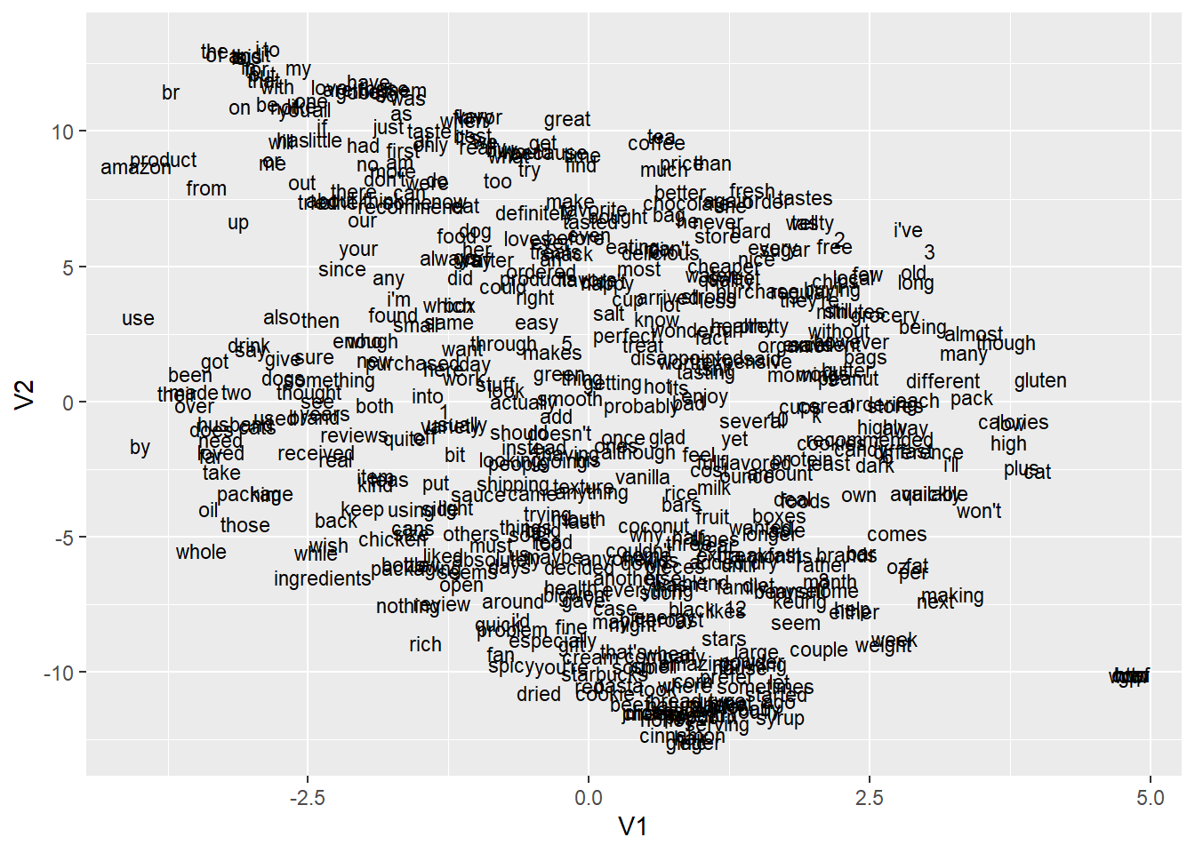

3.4.2 Using GloVe

source: http://text2vec.org/glove.html

In this example, we will use GloVe to test how much it captures linguistic regularities. By takig the word vectors corresponding to the words: “Paris”, “france”, and “gremany”, we are supposed to obtain “berlin” as closest resulting vector. \(vector("paris") - vector("france) + vector("germany")\)

we will use the wikpiedeia data which is used as a demo by wor2vec.

# download data
# download.file("http://mattmahoney.net/dc/text8.zip", "D:/NLP/NLP-book/data/text8.zip")
# unzip("D:/NLP/NLP-book/data/text8.zip", files = "text8", exdir = "D:/NLP/NLP-book/data/text8")
# load data
wiki = readLines("D:/NLP/NLP-book/data/text8/text8", n = 1, warn = FALSE)

Now, we create a vocabulary constituted of set of words for wich we want to learn word vectors.

# Create iterator over tokens
tokens <- space_tokenizer(wiki)
# Create vocabulary. Terms will be unigrams (simple words).
it = itoken(tokens, progressbar = FALSE)
vocab <- create_vocabulary(it)
str(vocab)

## Classes 'text2vec_vocabulary' and 'data.frame':  253854 obs. of  3 variables:
##  $ term      : chr  "aaaaaacceglllnorst" "aaaaaaccegllnorrst" "aaaaaah" "aaaaaalmrsstt" ...
##  $ term_count: int  1 1 1 1 1 1 1 1 1 1 ...
##  $ doc_count : int  1 1 1 1 1 1 1 1 1 1 ...
##  - attr(*, "ngram")= Named int  1 1
##   ..- attr(*, "names")= chr  "ngram_min" "ngram_max"
##  - attr(*, "document_count")= int 1
##  - attr(*, "stopwords")= chr 
##  - attr(*, "sep_ngram")= chr "_"

We should remove unbommon words since it is not meaningful to keep word vector for word that we saw only once in the entire corpus. In this example we will keep only ords which apear at least five times.

vocab <- prune_vocabulary(vocab, term_count_min = 5L)
min(vocab$term_count)

## [1] 5

Now we have 71,290 terms in the vocabulary and are ready to construct term-co-occurence matrix (TCM).

# Use our filtered vocabulary
vectorizer <- vocab_vectorizer(vocab)
# use window of 5 for context words
tcm <- create_tcm(it, vectorizer, skip_grams_window = 5L)
tcm[1:10, 1:10]

## 10 x 10 sparse Matrix of class "dgTMatrix"

##    [[ suppressing 10 column names 'aapke', 'ababda', 'abakumov' ... ]]

##                                   
## aapke       . . . . . . .    . . .
## ababda      . . . . . . .    . . .
## abakumov    . . . . . . .    . . .
## abalones    . . . . . . .    . . .
## abano       . . . . . . .    . . .
## abati       . . . . . . .    . . .
## abbates     . . . . . . 1.25 . . .
## abbesses    . . . . . . .    . . .
## abderus     . . . . . . .    . 1 .
## abdications . . . . . . .    . . .

Now we have a TCM matrix and can factorize it via the GloVe algorithm.

glove = GlobalVectors$new(rank = 50, x_max = 10)
wv_main = glove$fit_transform(tcm, n_iter = 10, convergence_tol = 0.01)

## INFO  [23:50:33.466] epoch 1, loss 0.1745 
## INFO  [23:50:47.080] epoch 2, loss 0.1224 
## INFO  [23:51:00.388] epoch 3, loss 0.1083 
## INFO  [23:51:13.728] epoch 4, loss 0.1004 
## INFO  [23:51:27.567] epoch 5, loss 0.0953 
## INFO  [23:51:40.924] epoch 6, loss 0.0917 
## INFO  [23:51:54.514] epoch 7, loss 0.0889 
## INFO  [23:52:08.667] epoch 8, loss 0.0868 
## INFO  [23:52:22.352] epoch 9, loss 0.0850 
## INFO  [23:52:35.699] epoch 10, loss 0.0836

dim(wv_main)

## [1] 71290    50

Note that model learns two sets of word vectors - main and context. Essentially they are the same since model is symmetric. From our experience learning two sets of word vectors leads to higher quality embeddings.

wv_context = glove$components
dim(wv_context)

## [1]    50 71290

While both of word-vectors matrices can be used as result it usually better (idea from GloVe paper) to average or take a sum of main and context vector:

word_vectors = wv_main + t(wv_context)

We can find the closest word vectors for our paris - france + germany example:

berlin = word_vectors["paris", , drop = FALSE] - 
  word_vectors["france", , drop = FALSE] + 
  word_vectors["germany", , drop = FALSE]
cos_sim = sim2(x = word_vectors, y = berlin, method = "cosine", norm = "l2")
head(sort(cos_sim[,1], decreasing = TRUE), 5)

##     paris    berlin      bonn    london   leipzig 
## 0.7771973 0.7295444 0.6742783 0.6663386 0.6612857

3.5 references

• http://pablobarbera.com/ECPR-SC105/code/16-word-embeddings.html
• https://code.google.com/archive/p/word2vec/
• https://m-clark.github.io/text-analysis-with-R/word-embeddings.html#wikipedia
• https://juliasilge.com/blog/gender-pronouns/
• https://machinelearningmastery.com/use-word-embedding-layers-deep-learning-keras/
• https://machinelearningmastery.com/what-are-word-embeddings/
• https://rpubs.com/JanpuHou/396443
• https://mran.microsoft.com/snapshot/2016-03-05/web/packages/text2vec/vignettes/text-vectorization.html
• https://cbail.github.io/textasdata/word2vec/rmarkdown/word2vec.html
• https://www.jla-data.net/eng/vocabulary-based-text-classification/
• http://text2vec.org/glove.html
• http://text2vec.org/similarity.html
• https://www.r-craft.org/r-news/get-busy-with-word-embeddings-an-introduction/